Job Search Part 4: Timing Beveridge Curve Movements During A Recession

This economics blogger feels like he would be cheating the reader if he did not include recent work done by Barnichon and Figura (2010) on timing movements in the unemployment rate during recessions. That is why this is part 4 of my special 5 part mini-series on the modern job search and matching theory of unemployment. 
         In recessions there are a series of events that take place in the labor market. Unlike market-clearing models, real life agents are not in fact homogeneous and do react over time rather than instantaneously.  At the beginning of a recession, the Beveridge curve shifts out because of an increase in temporary layoffs.  A quarter later, a clockwise rotation of the job creation curve moves unemployment along the Beveridge curve as firms adjust vacancies. The Beveridge curve also shifts out further because of an increase in permanent layoffs.  One quarter later the labor supply reacts and the Beveridge curve shifts in slightly as quits decline but shifts out further as workers display a stronger attachment to the labor force.  What follows is a graphical representation of the logical pattern of events that takes place during recessions. 
Figure A: Increase In Temporary Layoffs

Figure A describes the very beginning of a recession when there is an increase in the amount of temporary layoffs. The Beveridge curve shifts out from BC0 to BC1 because of an increase in temporary layoffs. The vacancy rate moves from V* to V1 and the unemployment rate increases from U* to U1 as we move from point A to B.
Figure B: Firms Cut Back Vacancies and Job Openings

In Figure B, we are one quarter later in time and see firms adjust to the recession by cutting back the amount of job availability and vacancies. This lowers the amount of tightness present in the labor market which rotates the job creation curve JC0 downward to JC1. The vacancy rate goes from V1 to V2 and the unemployment rate increases from U1 to U2 thus moving from point B to C.
Figure C: Increase in Permanent Layoffs

In Figure C, we are still in the same quarter as Figure B.  Because of an increase in permanent layoffs we see  an outward shift in the Beveridge curve from BC1 to BC2 which results in the unemployment rate increasing from U2 to U3 as we move from point C to D.
Figure D: Slight Decline in Quits

Figure D depicts the 3rd quarter of the recession where labor supply finally reacts to this debacle. The Beveridge curve shifts in slightly from BC2 to BC3 as quits decline.  This is understandable, in recessions uncertainty about the future is elevated, asset prices fall broadly so the wealth effect has a huge say and a job is considered a luxury so people feel the maybe I'll put off retirement until later effect.  The unemployment rate moves from U3 to U4 as we move from point D to E. 
Figure E: Workers have a stronger attachment to the labor force

Figure E is also in the 3rd quarter and shows an outward shift in the Beveridge curve from BC3 to BC4 as workers show a stronger attachment to the labor force. We move from point E to F and the unemployment rate increases from U4 to U5.
          While only suggestive, this chain of events could indicate that labor supply responds to labor demand at cyclical frequencies. When the job creation curve rotated downward it was all labor demand, and since it remained flat shifts in the Beveridge curve translated to almost a full increase in the unemployment rate by the same amount. Although labor supply responds to labor demand when we experience high amounts of volatility (either during expansions or contractions) over the long-run however unemployment is driven by secular changes in labor supply, specifically the aging of the baby boomers and the increasing attachment of women to the labor force.


Modeling The Influence of Labor Demand on Unemployment


In the above section we followed Barnichon and Figura (2010) work and arrived at the conclusion that at cyclical frequencies (during recessions and expansions) labor demand was the prime driver behind movements in the unemployment rate. I sought to test their theory by estimating movements in the Beveridge curve and the job creation curve from 12/01/2007 to 08/01/2009.  Pictured below are my results.
Figure F: Labor demand did dominate any movements in the unemployment rate during the recession

The data in the above figure comes from FRED, JOLTS and the BLS.
The first job creation curve has a slope θ = .5272 which is the mean of labor market tightness observations from 12/01/2007 to 05/01/2008. The second job creation curve has a slope θ = .16194 which is the mean of labor market tightness observations from 03/01/2009 to 08/01/2009. The power function was chosen to estimate the two Beveridge curves. For the complete details on how I derive the job creation and Beveridge curves please refer to my paper which can be found in the first post on the modern job search and matching theory of unemployment. 
Figure F clearly shows that the increase in unemployment quite overwhelmingly stemmed from labor demand conditions as embodied by the downward rotation of the job creation curve.  Notice that the Beveridge curve failed to shift in any significant way over this time period. 

Job Search Part 2: Minimum Wage Effects on Job-Search Effort and Labor Force Participation

In the previous post we built a solid foundation with the tools and terms of job search theory. Let's take what we've learned and apply it to analyzing the effects of an increase in the minimum wage.

Figure A: Conditions Before a Minimum Wage Increase

Assume that initially the wage-setting (WS0) and vacancy-supply (VS0) curves  intersect at point A determining both the equilibrium market wage w* and equilibrium labor market tightness, θ*. The job creation curve (whose slope is θ*) intersects our Beveridge curve at point A1 which determines that our equilibrium vacancy rate is V* and equilibrium unemployment rate is U*. These are represented graphically in Figure A.

Figure B: After a Mandated Increase in the Minimum Wage

Then out of the blue the government introduces a minimum wage w1 that exceeds the market wage w*.

The wage-setting curve now has a "floor" and this is represented by its vertical portion at the minimum wage.  As higher wages cut into business profits, firms open fewer vacancies. We move from point A to B in Figure B.   Since labor market tightness has now decreased from θ* to θ1, the job creation curve (with its new slope θ1) rotates downward.  The rotation of the job creation curve from JC0 to JC1 increases the unemployment rate from U* to U1. We moved from our original position at A1 to B1 and the job openings rate has decreased from V* to V1. In this situation a binding minimum wage raises both wages and unemployment. 

Incorporating Workers Job-Search Effort

Let's assume now that workers can choose the intensity with which they search for a job- how much time they spend searching the internet for a job, how many job applications they fill out, ect.  Under this assumption, a higher wage has two simultaneously opposing effects: 

a) A higher expected wage increases the payoff for workers when they finally do find a job. A worker with this in mind will be motivated to look harder and "more intensely." This increase in work intensity would shift our Beveridge curve inwards.
b) It weakens firms' incentives to create jobs because it cuts into their profit and thus making workers less likely to succeed and so depressing their search efforts.  Less intense search effort by the firm would correspond to an outward shift of the Beveridge curve.

        The net effect of these countering forces depends on where the wage stood before the increase.  To visualize this, consider two extreme cases where wages are initially really high or really low, depending on the extent of the workers bargaining power. First, suppose that workers are powerless and have no bargaining power, firms post wages unilaterally, and workers search until they find an acceptable wage offer.  Since employers appropriate the entire surplus from their relationship with labor, unemployed people have very little incentive to search actively for a job and the result is high unemployment.  Now consider the other extreme, where workers have all the bargaining power to set wages.  Firms make no profit from hiring more workers.  Since opening and advertising job vacancies is costly, firms rather not do so, and unemployment increases. 


Figure C: Increased Search Intensity by Workers

Markets that tend to be dominated by employers or equivalently where workers' bargaining power is pretty low, a compulsory increase in the wage can lead to higher search intensity and higher employment.  If the market wage is low, then a binding minimum wage can make employment more attractive to workers which strengthens their search efforts and reduces unemployment. Figure C graphs this result. The increase in workers search intensity would shift the Beveridge curve inward from BC0 to BC1 and the unemployment rate would go from U1 to U2, before the shift we were at point B1 and after the shift we settle at point C1.  In this respect the search model's results are consistent with the monopsony model as it explains how, in theory, a minimum wage can reduce unemployment.  If the the market wage is high, a binding minimum wage may discourage workers from looking for a job because there are fewer vacancies. It can also be shown that worker's search effort and social welfare move together.  The wage that maximizes search effort also maximizes social welfare. If the minimum wage is small enough, it can improve labor market conditions and increase social welfare.  
       Another interesting result of this model is that the minimum level of unemployment occurs when the market wage is below the one maximizes workers search effort.  This means that a minimum wage can make workers better off even if it increases unemployment.

Adding Labor Force Participation

If we focus our attention on the workers' decision to participate in the labor force we can use logic that mirrors that from our search intensity example.  If the market wage is very low because workers have little bargaining power, they might decide to not even look for a job at all.  They have no incentive to enter the market because non market activities, like home production and leisure, are more valuable than working and thus employment is low. Conversely if the market wage is very high, firms are not hiring, unemployment durations are long, and workers stay out of the labor force.  In general, employment is a hump-shaped function of the wage. However, unlike the model with workers' search effort, unemployment always decreases with the wage.  

         Although participation is weaker when wages are low, firms still create jobs because their profits are high.  This has the effect of swelling the number of vacancies relative to the number of job seekers, making it more probable that they will find employment.  If the market wage is too low and workers lack bargaining power, the introduction of a binding minimum wage strengthens labor force participation even though the duration of unemployment increases.  In contrast, if the market wage is high, a minimum wage reduces the supply of vacancies and increases unemployment duration, which has the balancing effect of discouraging workers from entering the labor force.      

Job Search and Matching Theory Part One: Building Blocks

When we hear or read about the labor market, we always see this debate and confusion over the types of unemployment (structural vs. cyclical) and the reasons underlying movement in the unemployment rate.  The modern job search theory of unemployment helps us to end the confusion by allowing us to logically analyze the labor market.  It helps us view the labor market as a liquid arena, where jobs are created, matches are made, and workers decide to enter or leave the labor force.  It is a constantly changing and evolving environment that has until pretty recently proved a conundrum wrapped in an enigma. The job search theory allows us to realistically break apart the unemployment rate in away we haven't been able to do before.  It's not just blanket defining structural unemployment, frictional unemployment and cyclical unemployment, guessing at which one matters more, and arriving at various highly opinionated conclusions.  This theory is empirically testable! We can see with our own beautiful eyes what is causing unemployment to rise and fall. 


That is why today I will begin a special mini-series of posts regarding The Modern Job Search Theory of Unemployment. The beginning posts will involve a very light historical perspective and then will dive into the heart of the theory.

Some Historical Perspective

The Beveridge curve is named after William Beveridge, a British Lord, lawyer, member of parliament and founder of the modern British state. Beveridge first discussed the relationship between labor demand captured by the vacancies and unemployment rate in a 1944 report titled, Full Employment In a Free Society. Although he refrained from explicitly plotting the relationship, he provided detailed data on the variables and discussed them at length. His work was the first to imply that there is a negative relationship between vacancies and the unemployment rate.  
His early contributions even tackled many of the issues that remain under study today. These include the potential mismatch between unemployed workers and job openings, trend versus cyclical changes in the unemployment rate, measurement issues, and aggregate demand versus reallocation factors.
The early literature of the late 1950's and the 1960's dealt with the Beveridge curve in the context of understanding excess demand in the labor market and its direct influence on wage inflation (Yashiv 2006). This is not surprising given how much attention was given to the Phillips curve.  In fact so much research was devoted to the Phillips curve that Janet Yellen once referred to the Beveridge curve as,"the neglected stepsister of macroeconomics."(More of Janet Yellen's thoughts as well as Robert E. Hall's thoughts on the Beveridge curve can be found Hall, R. E (1989).) As Eran Yashiv notes,

The literature typically defined excess demand as unfilled vacancies less unemployed workers, considered the data on these variables, and then looked at the relationship between measures of excess demand and wage behavior. (Yashiv 2006)

This literature acknowledged that even in the absence of excessive labor supply, unemployment would still persist due to frictions.  Contributions by Dow and Dicks-Mareaux (1950), Lipsey (1960), Holt and David (1966), Hansen (1970), and Bowden (1980), made much progress on the Beveridge curve.  According to Yashiv (2006) this literature derived,

A negatively sloped u-v curve from a model of distinct labor markets, interacting at different levels of disequilibrium, with the markets at points off both labor supply and demand curves. 

Furthermore, the u-v curve was shown to be static and stationary, and observed vacancy and unemployment rates were expected to cycle around it. Increases and decreases in the excess demand for labor were reflected in movements up and down the curve. Shifts in the curve were identified as changes in the speed of market clearing or changes in the sectoral composition of labor demand.
          In the 1970's and 1980's an alternative search and matching model approach was developed. An important difference between this model and the earlier stand of literature stems in its derivation of vacancies and unemployment as equilibria, as opposed to disequilibria phenomena. This model was developed with the combined efforts of Peter Diamond, Dale Mortensen and Christopher Pissarides.  


Dale T. Mortensen wrote in 1992 about a divergence in neoclassical macroeconomic labor theory. He stated that, (Mortensen also summarized the rest of search theory very nicely in "Search theory and macroeconomics: a review essay"(1992))

Two views were born out of Phelps (1970) volume:  An intertemporal generalization of the traditional income-liesure model of labor supply and an early version of what came to be known as the job-search model.  Subsequently, the Lucas-Rapping approach with its emphasis on intertemporal substitution and market clearing came to dominate the macroeconomic scene.  One reason for the lesser role played by the search-theoretic approach in macroeconomics was its partial-partial nature, specifically the absence of a consistent view of how the labor market operates when transaction cost and time lags are important in the job/matching process.

Although there was a lack of development early on, the realism embodied by the search model's characterization of the individual workers experiences moving in and out of employment and among jobs has  proved a substantially more valuable tool for empirically understanding the labor market than has intertemporal substitution. (Intertemporal substitution is used in Real Business Cycle models to describe the decisions workers must make between leisure and work for pay.  The logic goes like this: a higher a real interest raises the opportunity cost of sitting around because money is worth more so people respond by entering the labor force and when the real interest rate is lower then people leave the labor force because they value leisure and home production more so.)
It was in a 1971 paper, that Peter Diamond first showed that the mere presence of costly search and matching frictions prevented the law of one price from holding. Diamond found that even a minute search cost moves the equilibrium price far from the the competitive price and that the only equilibrium price was a monopoly one. This finding dubbed the "Diamond Paradox" has generated much additional research.  
           An additional issue with search markets is wether there is too much or too little search, or another way of phrasing this is, do markets deliver efficient outcomes or not? The economy undeniably has search frictions, so the relevant issue is not whether an economy is inefficient because of frictions, but rather is the economy constrained efficient i.e. delivers the optimal result, given these restrictions. Diamond, Mortensen and Pissarides all contributed important insights into the efficiency question with the first work appearing in the late 1970s and early 1980s. A standard result is that efficiency cannot be expected and policy interventions therefore become necessary.
           It was Christopher Pissarides that brought to light and demonstrated that the transactions approach to the labor market can serve as a useful framework for macro-labor analysis. He helped develop the idea of a matching function and pioneered the empirical work on its estimation. For a survey of the matching function please see Petrongolo and Pissarides (2001). 
           The sum of the research done by these three economists has fundamentally influenced our views on the workings of the labor market. A key contribution is the development of a new framework for analyzing labor markets both positive and normative questions. These resulting advancements are now known as the Diamond-Mortensen-Pissarides model (or the DMP model). The DMP model originated from the insights of the first search and matching models of the 1970s and other crucial developments followed. As the Economic Sciences Prize Committee of the Royal Swedish Academy of Sciences puts it:

The DMP model allows us to consider simultaneously (i) how workers and firms jointly decide whether to match or to keep searching; (ii) in case of a continued match, how the benefits from the match are split into a wage for the worker and a profit for the firm; (iii) firm entry, i.e., firms’ decisions to “create jobs”; and (iv) how the match of a worker and a firm might develop over time, possibly leading to agreed-upon separation.

The resulting models and their subsequent advances have been quite rich and the applied research on labor markets, both empirical and theoretical, has blossomed. Theoretical work includes both positive and normative economic analysis. This theory makes it relatively straightforward to examine the policy effects on hiring costs, firing costs, minimum wages laws, taxes and unemployment benefits on both unemployment and social welfare. 
Empirical work consists of ways to evaluate the search and matching model using aggregate date on vacancies and unemployment. This includes the development of data bases and analysis of labor market flows, such as the flows of workers between different types of employment. Moreover, the DMP model is used to analyze how aggregate shocks affect the labor market and lead to cyclical fluctuations in unemployment, vacancies and employment flows.  
           This model brought with it a level of practicality that had not been found in previous labor market theories.  Because of its focus on job flows into and out of employment and its potential to greatly enhance the way we analyze the labor market, the Bureau of Labor Statistics in 2000 started the Job Openings and Labor Turnover Survey (JOLTS) to specifically fit this model (Clark and Hyson 2001):

The JOLTS data series on job openings, hires, and separations will assist policy makers and researched in addressing some fundamental issues concerning labor demand and movements in the labor market.  The JOLTS data will provide a basis for improved understanding of the factors driving fluctuations in unemployment and the overall economy, determining appropriate approaches for reducing unemployment, and studying how workers flow in and out of establishments, are matched with job, and are distributed across sectors (pg. 33). 

With these time-series researchers are now able to make tangible and empirically test labor market search and matching theories.

The Labor Search and Matching Theory of Unemployment

The labor market is known to have problems clearing. Economists have long recognized this fact and attribute the labor markets inability to flawlessly and effortlessly match workers and jobs to “frictions”. These “frictions” occur because labor is not homogenous and instead labor has the fortunate or unfortunate quality of being heterogeneous. Being heterogeneous means that there is not one universal price that can be exchanged for one universal unit of labor. This makes it a market that acts much differently from other commodities, like gold whose “law of one price” attribute allows it to consistently clear. We are dealing with a commodity that can speak, feel, learn and prides itself of differentiation and individuality. The heterogeneity of labor makes it difficult for employers to distinguish the productive from the unproductive, and even the process of moving from one job to the next is not costless. The search and matching model of unemployment provides the theoretical groundwork for us to effectively model these frictions. 

The search and matching model contains three elements; setting wages, creating job vacancies and matching workers and jobs. The first element describes how wages are set through the bargaining process. The second element determines the number of job openings that firms make available, and the third ties them together in the act of creating jobs. 

Setting Wages

Although it is important to recognize that not all wages are determined in the same way, we can assume that many are the result of a bargaining process between workers and their employers. Additionally, it is really helpful to note here that unlike Walrasian theory, there is no unique equilibrium concept inherent in the theory of markets with transaction costs. Wages must be determined by some form of bargaining and the implications of the model are sensitive to which form of bargaining solution is imposed (Mortensen 1992). The bargaining process itself relies on the relative bargaining strength and outside options of both parties involved, which in our case is the potential employer and worker. The party with the most bargaining power can extract a larger fraction of the surplus that stems from their relationship. The outside options of these parties depends on their relative incomes if "unmatched" as well as their capacity to locate alternative resources if the negotiation falls through. Outside options are affected by labor market imbalances like the number of vacancies and the number of unemployed workers. Labor market tightness is what helps us determine this relative bargaining power. Labor market tightness is represented by:

θ ≡ vt/ut 

Where labor market tightness, θ ,  is defined as the number of vacancies vt at time t divided by the number of unemployed ut at time t. This θ, is a measure is a measure of worker scarcity and enables us to operationalize the idea of bargaining power.  It is this crucial element that lets us finally introduce the wage-setting curve.

The wage-setting curve, WS, is the positive relationship between a workers relative bargaining power which is represented by labor market tightness and the market wage.  Looking at Figure 1 it becomes evident that as labor market tightness increases, the bargaining strength of market participants shifts in the favor of workers and wages increase.

Additionally their bargaining is enhanced because they are presented with a larger array of possible alternatives for employment. This allows workers to request a higher wage and reflects movement up the wage-setting curve. 

           If the number of vacancies per unemployed worker is high, we are faced with a "tight" labor market where workers outside options are decent thus allowing them to ask for a higher wage.  Firms are willing to pay this high wage to avoid the hassle of finding another worker and incurring higher recruiting costs. On the flip-side, if vacancies are scarce relative to unemployed workers, we have a "loose" labor market where workers outside options are poor thus increasing their willingness to accept a lower wage to avoid a long spell of unemployment. 

Figure 1: A rightward shift of  the Wage-Setting Curve

The wage-setting curve shifts whenever the economic fundamentals change.  

Factors that shift the wage-setting curve include:

a). Changes in worker productivity (+) 

b). Changes in worker bargaining power (+)

c). Changes in unemployment benefits (+)

Rightward shifts from WS1 to WS2 would be caused by increases in worker productivity, worker bargaining power and unemployment insurance benefits.

Vacancy Supply and Job Creation

We will now focus on determining the number of workers that firms want to hire. If a firm found workers instantaneously and with zero recruiting cost, they would continue hiring workers as long as each new worker's productivity exceeded the market wage.  Since hiring a worker is neither costless or instantaneous there must exist market frictions. 

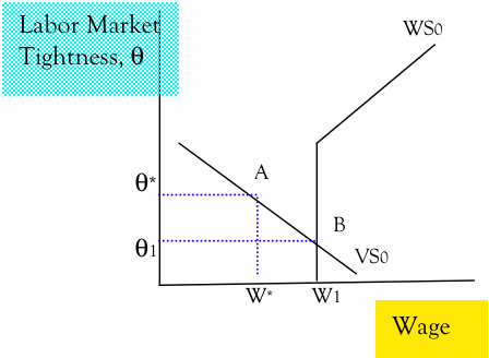
Various frictions include promoting job openings and evaluating potential candidates. A firm will want to make a job opening available if the sum of profits it makes from hiring compensates for the recruiting expenses. This is referred to as the vacancy-supply condition and is represented by the downward sloping curve VS that is in Figure 2.  It is interesting to note that the Vacancy-Supply curve replaces the labor demand curve found in standard Walrasian theory.   

It says that the number of vacancies opened in a labor market is determined as a function of the market wage ,w, and recruiting costs. The downward relation is intuitive, firms have less incentive and ability to create jobs as the market wage increases. 

At lower wages, workers generate higher profits, and firms are willing to open a large number of vacancies. As the number of vacancies increases it becomes more challenging for firms to find employees. As a result, hiring and recruiting costs increase until the incentives to open up new vacancies disappears.

Figure 2: Upward Shift of the Vacancy-Supply curve

Shifts in the vacancy-supply curve stem from changes in labor market fundamentals. The vacancy-supply curve shifts upward, as in Figure 2, whenever firms want to hire more workers and therefore offer more job openings. Factors that shift the vacancy-supply curve upward from VS1 to VS2 include:

a.) Increase in worker productivity 

b.) Decrease in cost of advertising vacancies and recruitment

c.) Process of finding workers becomes more efficient

The intersection of the wage-setting and vacancy-supply curves is what determines the labor market tightness θ and market wage, w.  The determination of labor market tightness is what provides the essential link for determining the equilibrium unemployment rate and job openings. 

Matching Workers with Jobs

In the previous two sections we gave a brief overview of the wage-setting and vacancy-supply curves and determined that their intersection provides us with two important links, labor market tightness and the market wage.  

To get a complete picture of the labor market however, we will need to incorporate two last items: the unemployment rate and the vacancy rate. These two things in relation to each other and labor market tightness will lead us to the derivation of the equilibrium unemployment and vacancy rate. To make this connection it is required that we understand how the number of vacancies affects unemployment, which requires that we develop an understanding of how vacancies and unemployed workers are matched to create jobs. 

Frictions have been used to explain unemployment in the labor market. In the majority of cases, the modeling tool preferred to capture the influence of frictions on equilibrium outcomes is the aggregate matching function. The matching functions appeal is that it enables the modeling of frictions to be added to conventional models, but with a very minimal amount of added complexity (Petrongolo and Pissarides 2001). Frictions stem from asymmetric information, heterogeneities, slow mobility, congestion from large numbers, and numerous other factors. The matching function captures the frictions cumulative effects on equilibrium in terms of a very small number of variables, and usually without explicit reference to the source of the frictions. Petrongolo and Pissarides (2001) explain the key idea very well,

The matching function summarizes a trading technology between agents who place advertisements, read newspapers and magazines, go to employment agencies, and mobilize local networks that eventually bring them together into productive matches.  The key idea is that this complicated exchange process is summarized by a well-behaved function that gives the number of jobs formed at any moment in time in terms of the number of workers looking for jobs, the number of firms looking for workers, and a small number of other variables.

This matching process is called a productive process and has one output and two inputs. The one output is the number of jobs created through the matching process and the two inputs are the number of unemployed and the number of job openings. The relationship between the stock of unemployed and the stock of vacancies to the number of jobs created is the matching function. The matching function in equation form is as follows:

H = xt* M(Lu , Lv ) 

Where, H= new hires, Lu_t = Unemployment (it's the unemployment rate times the labor force) and Lv_t= the number of vacancies (it's a vacancy rate v=(Vacancies\ Labor Force) times the labor force). xt = Total Factor Productivity and also known as the "Solow Residual".  We can estimate the matching function using a Cobb-Douglas production function.  The Cobb-Douglas works well as the proper matching function because it has constant returns to scale.  Constant returns to scale means that doubling the inputs yields double the output.  According to Pissarides (2000) the reason constant returns to scale are assumed is because "It is empirically supported and plausible, since in a growing economy constant returns ensures a constant unemployment rate along the balanced-growth path" pg.6 We can estimate the following matching function:

M (Lu, Lv) = Lu^α*Lv^(1-α)

Where, α + (1 − α) = 1

Next I use the JOLTS data to compute the matching function "Solow residual". We assign α =.5 so 1-α = .5. Next I take the log of the Cobb-Douglas production function:

log(x)=log(H) −0.5log(Lu)−0.5log(Lv) 

I do this In the style of  David Andolfatto who is the V.P. of Research at the St. Louis Federal Reserve and also author of a marvelous blog named MacroMania.  The following data sets from FRED were used over the time span 12/01/2007 to 06/01/2009, JTSJOL Job Openings: Total Nonfarm (JTSJOL), Level in Thousands, Monthly, Seasonally Adjusted

UNEMPLOY Unemployed (UNEMPLOY), Thousands, Monthly, Seasonally Adjusted, JTSHIL Hires: Total Nonfarm (JTSHIL), Level in Thousands, Monthly, Seasonally Adjusted. Figure 3 plots the results of the above equation in log form.

Figure 3: Matching Function TFP

A quick glance at Figure 3 reveals that total matching function efficiency  from the beginning of the recession to the very end declined by about 35 percent. I use the official NBER dating of the recession which can be found at  http://www.nber.org/cycles.html. Obviously thats a pretty substantial decline, but how does that impact the big picture? Changes in matching efficiency play on average a pretty small role but can decline substantially during recessions. In fact, between 2008 and 2009, lower matching efficiency added about 1 1/2 percent to the unemployment rate (Barnichon and Figura 2010). 

The matching function is depicted below in Figure 4. Unemployed workers and vacancies meet each other which feeds a flow of job creations into the stock of employed workers.  The stock of unemployed workers and the stock of vacancies are both replenished by job destructions. If the economy were not subject to shocks, it would end up in a steady state.

Figure 4: Job Flows

The number of jobs created equals the number of jobs destroyed and the stock of unemployed workers would remain unchanged.  In this steady state the unemployment rate would be low if the flow of job creations were large relative to job destructions. The flow of job creations is large relative to job destructions when the number of vacancies is large. In contrast, if there were few vacancies then the flow of job creations would be small, and the unemployment rate would be high. 

Although Figure 4 does a good job of giving a nice explaination of matching between unemployed workers and the available job openings, it is rather naive.  For example, workers are often encouraged to move from one job to another to increase their lifetime earnings potential. This flow is significant and for the United States is estimated to account for around 15 percent of job creation. That leaves the other 85 percent of new job creation to stem from those that are unemployed  and those moving from out of the labor force directly into employment.  A quick glance at the diagram shows that neither the flow to new matching from employment or from out the labor force is accounted for.  As for the rest of the 85 percent, it is estimated that 45 percent of that stems from those in the unemployment stock while the other 40 percent are from outside the labor force (These are the estimates produced by Blanchard and Diamond (1989))  

Within the United States the flow of hires from outside the labor force and those moving from job to job are both said to be procyclical. 

The figure does still however lead us to the intuition that the more job openings made available, the more job creation that can take place, and hence the lower the unemployment rate will be. The negative relationship between vacancies and unemployment (in our static steady state) is called the Beveridge Curve. The Beveridge curve was named after Lord William Beveridge who in the 1940's first identified the relationship between vacancies and unemployment (Bleakley and Fuhrer (1997). On another interesting note Janet Yellen, referred to the Beveridge curve as the, "neglected stepsister of macroeconomics."(More of Janet Yellen's thoughts as well as Robert E. Hall's thoughts can be found Hall, R. E (1989).  If the Beveridge curve was the neglected stepsister it was because her more flashy sister the Phillips curve was falsely getting all the attention.)

The Beveridge curve is where equilibrium unemployment is determined. Along the Beveridge curve the flows into and out of employment are balanced. The negative slope reflects the the dependence of unemployment duration on labor market tightness. It is important to realize that variables which shift the Beveridge curve to the right also increase equilibrium unemployment.

As Figure 5 demonstrates, movements along the Beveridge curve reflect cyclical factors. Recessions are often characterized by low vacancies and high unemployment which corresponds to the lower right hand branch of the curve.  The upper left hand side is characterized by expansions because these are generally times with many vacancies and a lower unemployment rate. Movements along the curve, from left to right are recessions and the subsequent recovery swing’s back up the other way.

Figure 5: The Beveridge and Job Creation Curve

Additionally, movements along the downward sloping Beveridge curve are typically

characterized as cyclical movements in the labor market, while persistent inward and

outward shifts in the curve are frequently attributed to overall labor market activity.  This is sometimes interpreted as the intensity of "reallocation", which is movement of workers from one job to the next and even from one sector to another within the economy.  

You may notice that Figure 5 has a line called Job Creation intersecting the Beveridge curve. Where the job creation curve and Beveridge curve intersect is where equilibrium frictional unemployment is determined.  The slope of the job creation curve is the labor market tightness  θ, that we determined from the intersection of the wage-setting and vacancy-supply curves.  This is what ties our analysis of the labor market all together.

The job creation curve rotates clockwise and counterclockwise whenever there is a change in labor market tightness. Changes in labor market tightness stem from shifts in the wage-setting and vacancy-supply curves.  Whenever the labor market becomes less tight the job creation curve rotates clockwise and when there is an increase in labor market tightness the job creation rotates counterclockwise. The job creation curve is upward sloping because as the the pool of the unemployed grows, employers can more easily fill open vacancies; this reduction in hiring costs leads to more vacancies being posted. Asking a question about the current position of the job creation curve is equivalent to asking "How much tightness is currently found within the labor market?" Well if we divide job openings by the number of unemployed we get Figure 6. What this graph shows us is that labor market tightness peaked around August 2007 before falling off and declining from 70 percent to about 15 percent.

Figure 6: Labor Market Tightness from March 2001 to January 2011

Another crucial insight is that the job creation curve represents the labor demand curve. With that in mind it rotates when there are changes in the cyclical components that affect the unemployment rate.

What might lead to a rise in the equilibrium unemployment rate?

This can be caused by an outward shift in the Beveridge curve, a downward shift in the job creation curve or a combination of both. First consider an outward shift in the Beveridge curve from BC0 to BC1 as depicted in Figure 7.

Figure 7: Outward shift in the Beveridge curve

For a given job creation curve this shift increases the equilibrium unemployment rate from U* to U1 and me move from point A to point B. Because the job creation curve is upward sloping equilibrium unemployment increases by less than the outward shift of the Beveridge curve, to a degree that depends on the the slope of the job creation curve which as we already know is labor market tightness θ. In order for the unemployment rate to increase by the same amount as the rightward shift in the Beveridge curve the job creation curve must either be flat or must simultaneously rotate downward.

Figure 8:Clockwise rotation of the Job Creation curve

This is represented in Figure 8, which shows that unemployment will only increase by the full amount of the shift in the beveridge curve if the job creation curve does a clockwise rotation. Notice how much more the unemployment rate increases if it is accompanied by a flat or rotating job creation curve. Instead of ending up at B and U1 as in Figure 7 the unemployment rate ended up all the way at U2 at point c.  

Given our ability to derive the job creation curve from the vacancy-supply and wage-setting curve it would now be nice to see what shifts the Beveridge curve. We need to distinguish what part of the rise in the unemployment rate reflects cyclical fluctuations in labor demand (or the job creation curve) and what part is due to other transitory or permanent factors. We will now discuss some of the known causes of shifts in the Beveridge curve.

Figure 9: Rightward Shift in the Beveridge Curve

Shifts in the Beveridge curve for any given labor market tightness can be caused by each of the following:

a). The matching process will determine how efficiently workers find new jobs and thus determine the position of the Beveridge curve.  Increased matching efficiency shifts the curve inward and vice-versa. Increased matching efficiency can come from many sources which includes the use of internet job sites, more temporary help service centers and help from One-Stop Career Centers. Additionally lower union participation rates and increased labor mobility are also found to increase matching efficiency. Increased mobility of labor is also a way of saying a reduction of barriers to mobility which include both geographical and occupational factors. Generous unemployment insurance benefits may also slow down the matching process but more information will be deferred to our example that will be presented in a later post.

b). Changes in the labor force participation rate will shift the Beveridge curve. One example of something that would shift the curve outward is an increase in the labor force participation rate (Please see DiCecio, Riccardo and Charles S. Gascon, “Vacancies and Unemployment,” Federal Reserve Bank of St. Louis Economic Synopses; 2009. Number 44). As new workers enter the labor market, they join the ranks of the unemployed searching for work. Higher levels of labor force growth translates to greater unemployment, since more workers are searching for jobs at any particular time.  In the short-run, vacancies may not fully adjust to an increase in labor force growth.  In the long-run however, vacancies will increase roughly in line with unemployment (Bleakley and Fuhrer 1997). Additionally, labor force participation increases when more people are educated and as immigration increases.

c). Average duration of unemployment will shift the Beveridge curve. Long-term unemployment will force the curve outward because those unemployed face human capital deterioration and loss of skill.  Employers negative perception of these workers may lead them to consider a less experienced and cheaper college graduate when making a hiring decision.

d). A change in the degree of "churning" in the labor market will shift the Beveridge curve. Job loss, quits, and job creation is related to the overall pace of reallocation or "churning" in the economy.  Reallocation occurs even when the economy is stable, as some firms expand and others contract for firm or industry-specific reasons.  The pace of reallocations increases during recessions and in fast expansions as firms are driven to contract or expand significantly, which leads to both greater flows of workers and jobs.  Thus, changes in the pace of reallocation imply potentially large movements in the gross flows of the labor market- flows into and out of employment.  More churning implies lower average job tenure, higher turnover and more time spent moving among firms (or even sectors) in the economy.  An increase in churning means that each month more workers flow into unemployment and new vacancies are posted.  Such an increase would shift the Beveridge curve outward (Bleakley and Fuhrer 1997).  

e). Changes in worker and employer search intensity will impact matching efficiency and cause shifts in the Beverage curve. Increased search intensity by workers and recruiters alike will improve matching efficiency and shift the beverage curve inward.  Decreased search intensity by workers and recruiters will lessen matching efficiency and shift the Beveridge curve outward for any given labor market tightness.

f). The availability of credit and the presence of credit-constraints will shift the Beveridge curve.  In recessions many of the unemployed find themselves in a credit constrained position because of uncertainty in the financial markets.  Credit constraints are found to have a large impact on job search intensity which may explain an outward shift of the Beveridge curve.  The less money available to the job searcher the less intense the job search will be, especially if the credit availability is a crucial component to paying down a mortgage which would impact the workers mobility.            

g). Changes in "House Lock" shifts the Beveridge curve. House lock prevents mobility by job searchers. People who find themselves underwater on their mortgages (negative equity) may find it difficult to move, especially after a housing bubble. An increase in house lock shifts the Beveridge curve out to the right, increased mobility of homeowners shifts it to the left. Empirically, the effects of house lock have been found to be very minimal. 

Up till this point, we have explained the three building blocks of labor search theory.  The point where the wage-setting curve intersects the vacancy-supply curve determined both the going market wage w and the vacancy-unemployment ratio. The vacancy-unemployment ratio is referred to as labor market tightness. Labor market tightness determines the slope of the job creation curve, whose intersection with the Beveridge curve derives the unemployment rate.  

Next time we will delve into some applications, the first of which will involve the minimum wage and search intensity.