Monetary Policy and Credit Easing pt. 6: Empirical Estimation and Methodology

IT is now appropriate to lay out our two regression models in full for empirical estimation over our two separate time periods. The first estimation is from 4/1/71 to 7/1/97 and the second is from 4/1/01 to 4/1/11. The methodology employed in the estimation of these two models is a procedure using Generalized Least Squares with a Cochrane-Orcutt, style iterated residual value.  For those that wish to perform the same regressions at home I have provided the following links to my data.  This is for the estimation period from 1971 to 1997 and this one is for the 2001 to 2011 estimations. The following four steps were taken for each estimation:

1. Estimate the OLS regression

2. Fit OLS residual to an AR(p) process using the Yule-Walker Method and find the value of p.

3.  Re-estimate model using Generalized Least Squares fit by Maximum Likelihood estimation, using the  estimated p from 2, as the order for your correlation residual term.

4. Fit the GLS estimated residuals to an AR(p) process using the Yule-Walker Method and use the estimated p's as the final parameter estimates for the error term.

The end goal of the above procedure is to have our models be asymptotically BLUE or the Best Linear Unbiased Estimators.  The implies that they have the smallest variance out of all the models that meet the rest of the Gauss-Markov assumptions.  A little background behind the methodology is in order.  First we will perform the standard Ordinary Least Squares (OLS) regression on our dependent variables.  This will give us at the very least unbiased estimators.  Second we take the residuals from the first step and fit them to an AR(p) process as selected by the Yule-Walker Method.  This method selects the optimal lag that characterizes the autocorrelation in the residuals.  We automatically take this step, due to the well known fact that most time-series suffer from autocorrelation problems as verified by our correlograms.  Then we re-estimate the regression using Generalized Least Squares which adjusts each term and divides them by their individual variances, while also incorporating the AR(p) lag that we discovered during the previous step.  The final step, which fits our GLS models residuals to an AR(p) process is what leads to our asymptoticly efficient results. We lay out our first estimation period models below.

First Estimation:  4/1/71 to 7/1/97 

1. Monetary Policies Impact On Short-term Risk Premiums

Our first model which seeks to answer how monetary policy impacts the risk premia on short-term commercial paper as estimated over our first time period 4/1/71 to 7/1/97 is as follows:

SR^{premium}_{t}=ß_{0}+ß_{1}*FedBalance^{size}_{t}+ß_{2}*Support_{t} + ß_{3}*UGAP_{t}+ ß_{4}*FF_{t}+ ß_{5}*ER_{t}+ ß_{6}*YC_{t}+ ß_{7}*Default^{spread}_{t}+ ß_{8}*CP_{t}+ ß_{9}*OGAP_{t} + ß_{10}*FedGDP_{t}+ ß_{11}*govcredit_{t}+ ß_{12}*ForeignDebt_{t} +  µ_{t}

Where,

SR^{premium}_{t} = Short-term Risk Premium at time, t

Support_{t}= Fed's funds at depository institutions as a percentage of their main financing streams at time, t

FedBalance^{size}_{t}=  The Fed's credit market asset holdings as percentage of the total credit market assets at time, t

FF_{t}= Federal Funds rate at time, t

ER_{t}= Excess Reserves of Depository Institutions at time, t

YC_{t}= Yield curve at time, t

Default^{spread}_{t}= Default Spread between BAA_{t} & AAA_{t} rated bonds at time, t

CP_{t} = Corporate Profits After Tax at time, t

FedGDP_{t}= Fed's holdings of total public debt as a percentage of GDP at time, t

govcredit_{t}= Government Holdings Of Domestic Credit Market Debt As A Percentage Of The Total at time, t

ForeignDebt_{t}= Foreign Holdings of Federal Debt As A Percentage Of The Total at time, t

UGAP_{t} = Unemployment gap at time, t

OGAP_{t} = Output gap at time, t

µ_{t}= error term at time, t

R DATA WORK

So now it is time for the long awaited econometrics work in R. First thing you'll want to do is read the data into R from your data file which is in this case is the Earlreg file.

> earl<- read.csv("/Users/stevensabol/Desktop/R/earlreg.csv",header = TRUE, sep = ",")

Then you define your variable names so you can easily manipulate your data in R. So when you open the official .csv data file take a look at the variable names and rename them using the following procedure.  

>yc1<-earl[,"yc"]

After you define what you call everything you're then free to go crazy and run regressions.  Below is how you run the standard Ordinary Least Squares regression.  The lm function enables you to run linear regressions:

1. Estimate the OLS regression

>srp1.lm=lm(srp1~yc1+CP1+FF1+default1+Support1+ER1+FedGDP1+FedBalance1+govcredit1+ForeignDebt1+UGAP1+OGAP1)

In order to get the output you have to use the summary function:

> summary(srp1.lm)

Call:

lm(formula = srp1 ~ yc1 + CP1 + FF1 + default1 + Support1 + ER1 + 

    FedGDP1 + FedBalance1 + govcredit1 + ForeignDebt1 + UGAP1 + 

    OGAP1)

Residuals:

     Min       1Q   Median       3Q      Max 

-1.04289 -0.20145 -0.04041  0.15230  1.21044 

Coefficients:

               Estimate Std. Error t value Pr(>|t|)    

(Intercept)  -2.7591194  1.0359966  -2.663  0.00912 ** 

yc1           0.1320996  0.0580500   2.276  0.02516 *  

CP1          -0.0022773  0.0073773  -0.309  0.75825    

FF1           0.1699788  0.0340654   4.990 2.81e-06 ***

default1      0.4382965  0.1876685   2.335  0.02167 *  

Support1      2.2383850  0.6660140   3.361  0.00113 ** 

ER1           0.3351508  0.3017644   1.111  0.26959    

FedGDP1       0.3031938  0.2558144   1.185  0.23895    

FedBalance1   0.4014920  0.3477547   1.155  0.25124    

govcredit1   -0.0928817  0.0401603  -2.313  0.02294 *  

ForeignDebt1 -0.0068900  0.0215393  -0.320  0.74977    

UGAP1        -0.0912273  0.0520491  -1.753  0.08295 .  

OGAP1         0.0006669  0.0014895   0.448  0.65536    

---

Signif. codes:  0 ‘***’ 0.001 ‘**’ 0.01 ‘*’ 0.05 ‘.’ 0.1 ‘ ’ 1 

Residual standard error: 0.3789 on 93 degrees of freedom

Multiple R-squared: 0.6474, Adjusted R-squared: 0.6019 

F-statistic: 14.23 on 12 and 93 DF,  p-value: 2.642e-16 

Next we perform step 2 which is:

2. Fit OLS residual to an AR(p) process using the Yule-Walker Method and find the value of p.

> srp.lmfit<-ar.yw(srp1.lm$res)

> srp.lmfit

Call:

ar.yw.default(x = srp1.lm$res)

Coefficients:

     1  

0.2535  

Order selected 1  sigma^2 estimated as  0.1201 

So the Yule-Walker methodology fits the residual series to an AR(1) process.

3.  Re-estimate model using Generalized Least Squares fit by Maximum Likelihood estimation, using the  estimated p from 2, as the order for your correlation residual term.

In order to run a GLS regression your going to need to load the nlme package:

> library(nlme)

Then you can go crazy:

>srp1.gls=gls(srp1~yc1+CP1+FF1+default1+Support1+ER1+FedGDP1+FedBalance1+govcredit1+ForeignDebt1+UGAP1+OGAP1, corr=corARMA(p=1,q=0),method="ML")

> summary(srp1.gls)

The following output is produced:

Generalized least squares fit by maximum likelihood

  Model: srp1 ~ yc1 + CP1 + FF1 + default1 + Support1 + ER1 + FedGDP1 + FedBalance1 + govcredit1 + ForeignDebt1 + UGAP1 + OGAP1 

  Data: NULL 

       AIC      BIC    logLik

  100.7905 140.7421 -35.39526

Correlation Structure: AR(1)

 Formula: ~1 

 Parameter estimate(s):

      Phi 

0.3696665 

Coefficients:

                  Value Std.Error   t-value p-value

(Intercept)  -3.0219486 1.2595942 -2.399145  0.0184

yc1           0.1929605 0.0640627  3.012054  0.0033

CP1          -0.0060642 0.0071791 -0.844700  0.4004

FF1           0.1918066 0.0362894  5.285466  0.0000

default1      0.5292204 0.2060591  2.568293  0.0118

Support1      2.1086204 0.7405128  2.847514  0.0054

ER1           0.5651430 0.2770125  2.040135  0.0442

FedGDP1       0.1028773 0.3143122  0.327309  0.7442

FedBalance1   0.7845392 0.4130914  1.899190  0.0606

govcredit1   -0.1240196 0.0524191 -2.365922  0.0201

ForeignDebt1  0.0009822 0.0278623  0.035252  0.9720

UGAP1        -0.1266050 0.0657633 -1.925161  0.0573

OGAP1        -0.0014094 0.0014328 -0.983623  0.3279

 Correlation: 

             (Intr) yc1    CP1    FF1    deflt1 Spprt1 ER1    FdGDP1 FdBln1 gvcrd1

yc1          -0.267                                                               

CP1           0.054 -0.062                                                        

FF1          -0.308  0.726 -0.012                                                 

default1      0.081 -0.208  0.235 -0.342                                          

Support1     -0.005 -0.109 -0.107 -0.419  0.137                                   

ER1          -0.208  0.077 -0.081  0.067 -0.180  0.028                            

FedGDP1      -0.728 -0.059 -0.048  0.083 -0.057 -0.002 -0.308                     

FedBalance1   0.461  0.250  0.020  0.208  0.036 -0.081  0.445 -0.887              

govcredit1   -0.570 -0.233 -0.095 -0.291 -0.261  0.072  0.068  0.666 -0.784       

ForeignDebt1 -0.475  0.132  0.006 -0.092  0.093  0.219  0.057  0.059 -0.045  0.227

UGAP1        -0.048 -0.193 -0.062  0.085 -0.447  0.150  0.090  0.045  0.064 -0.053

OGAP1        -0.029  0.092  0.295  0.062 -0.208 -0.024  0.053 -0.021  0.013  0.056

             FrgnD1 UGAP1 

yc1                       

CP1                       

FF1                       

default1                  

Support1                  

ER1                       

FedGDP1                   

FedBalance1               

govcredit1                

ForeignDebt1              

UGAP1        -0.016       

OGAP1         0.064  0.041

Standardized residuals:

        Min          Q1         Med          Q3         Max 

-3.08026826 -0.62589269 -0.08409222  0.39781537  3.24233325 

Residual standard error: 0.3634024 

Degrees of freedom: 106 total; 93 residual

After you perform this step you have to refit the residuals in order to get serially uncorrelated terms.  

4. Fit the GLS estimated residuals to an AR(p) process using the Yule-Walker Method and use the estimated p's as the final parameter estimates for the error term.  

> s1glsres.ar<-ar.yw(srp1.gls$res)

> s1glsres.ar

Call:

ar.yw.default(x = srp1.gls$res)

Coefficients:

     1  

0.3718  

Order selected 1  sigma^2 estimated as  0.1163 

In order to see the results of these actions please refer to image below:

The Ljung-box Q is a test for autocorrelation between the lags in the error terms. Ideally in order to meet the BLUE criteria we have to reject the the null hypothesis for autocorrelation at each lag.  We can see that both our original OLS  and GLS estimations fail to pass the Ljung-Box Q. However when we readjust the error terms the final time we get residuals that are serially uncorrelated with each other.  

In order to get the above graph you have to first load the package that will allow you to perform the Ljung-Box Q plot:

> library(FitAR)

Then you can proceed from there and define how many plots should be in one picture.  In the above image we have 9 therefore:

> par(mfrow=c(3,3))

Then you can start adding in your plots.  Below is the code for producing the plots for the fitted GLS residuals.

> acf(s1glsres.ar$res[-(1)])

> pacf(s1glsres.ar$res[-(1)])

> LBQPlot(s1glsres.ar$res[-(1)])

We include the [-(1)] because exclude the first observation since we have an AR(1) process.

The same steps above can be applied to any time-series regression model.  In the next post we will discuss how to get some summary statistics.  Please keep dancin'

Steven J.

Monetary Policy & Credit Easing pt. 5: Explanatory Variables Continued...

Capturing Treasury Supply Effects

WE will need to account for things other than the Fed that influenced risk premia as they relate to Treasury supply. The following three variables are meant to accomplish such a thing:

1. Federal Reserves holdings of total public debt as a percentage of GDP

2. Total government holdings of domestic credit market debt as a percentage of the total

3. Foreign holdings of government debt as a percentage of total public debt

1. Fed's holdings of total public debt as a percentage of GDP

Federal Reserve holdings of total public debt as a percentage of GDP is important because it controls for how much Federal Government support the Fed is accounting for.  It is especially pertinent to our second estimation as the Feds holdings of total public debt relative to GDP increased sharply.  Operationally, we define this variable as:

FedGDP_{t}= {GovDebt_{t}^{Fed}\ GDP_{t}}x 100

Where,

GovDebt_{t}^{Fed}=Federal Debt Held by Federal Reserve Banks (FDHBFRBN) at time, t

GDP_{t} = Gross Domestic Product, 1 Decimal (GDP) at time, t

We expect that this variable will move in line with both short-term and long-term risk premiums. Therefore:

H_{0}: ß ≤ 0 vs. H_{a}: ß > 0

Data Issues

The time-series necessary for this variable is provided by FRED and the details are as listed:

(a) Federal Debt Held by Federal Reserve Banks (FDHBFRBN), Quarterly, End of Period, Not Seasonally Adjusted, 1970-01-01 to 2011-0
(b) Gross Domestic Product, 1 Decimal (GDP), Quarterly, Seasonally Adjusted Annual Rate, 1947-01-01 to 2011-07-01

2. Government Holdings Of Domestic Credit Market Debt As A Percentage Of The Total

It would be wise to include a variable that account for fiscal policies support of the financial markets.  This we can define as Federal Government holdings of credit market assets as a percentage of the total outstanding. To account for total government support of the financial markets we will use the following variable: govcredit.

govcredit_{t}={ CAssets_{t}^{Gov}\ CAssets_{t}^{Total} }x 100

Where,

CAssets_{t}^{Gov} = Total Credit Market Assets Held by Domestic Nonfiancial Sectors - Federal Government (FGTCMAHDNS) at time, t

CAssets_{t}^{Total} = Total Credit Market Assets Held by Domestic Nonfiancial Sectors (TCMAHDNS) at time, $t$

We expect that this variable will reduce both short-term and long-term risk premiums. Therefore:

H0: ß ≥ 0 vs. Ha: ß < 0

Data Issues

The time-series necessary for this variable is provided by FRED and the details are as listed:

(a) Total Credit Market Assets Held by Domestic Nonfiancial Sectors - Federal Government (FGTCMAHDNS), Quarterly, End of Period, Not Seasonally Adjusted, 1949-10-01 to 2011-04-01
(b) Total Credit Market Assets Held by Domestic Nonfiancial Sectors (TCMAHDNS), Quarterly, End of Period, Not Seasonally Adjusted, 1949-10-01 to 2011-04-01

3. Foreign Holdings of Federal Debt As A Percentage Of The Total

This variable labeled ForeignDebt_{t} seeks to capture the impact that foreign holdings of United States government debt have on both short-term and long-term risk premia.  Theory would suggest that as foreign holdings go up risk-premia would go down. Operationally this variable is defined as follows:

ForeignDebt_{t} = {GovDebt_{t}^{Foreign}\ total public debt_{t}} x 100

Where,

GovDebt_{t}^{Foreign}= Federal Debt Held by Foreign & International Investors (FDHBFIN) at time, t

total public debt_{t}= Federal Government Debt: Total Public Debt (GFDEBTN) at time, t

Our ß coefficient on this variable is expected to be negative for both short-term and long-term risk premia and therefore:

H_{0}: ß ≥ 0 vs. H_{a}: ß < 0


Data Issues

The following data comes from FRED and the details are as follows:

(a) Federal Debt Held by Foreign & International Investors (FDHBFIN), Quarterly, End of Period, Not Seasonally Adjusted, 1970-01-01 to 2011-04-01
(b) Federal Government Debt: Total Public Debt (GFDEBTN), Quarterly, End of Period, Not Seasonally Adjusted, 1966-01-01 to 2011-04-01

Accounting For Cyclicality

We include two variables to help account for cyclicality in the overall economy.  Both are relevant as the Fed uses these variables in its decision making process.  For example in setting the federal funds rate, the Fed is said to have used a Taylor Rule that incorporated both the output gap and unemployment gap in its objective function.  Thus incorporating these variables may present a problem of endogeneity over a short-part of our sample(like when a taylor-rule was said to be used), but these effects we will choose to ignore.  The two cyclical variables we shall use are the output gap and the unemployment gap. The output gap is defined,

OGAP_{t}= Potential GDP_{t} – GDP_{t} at time, t

Where,

Potential GDP_{t}=Nominal Potential Gross Domestic Product (NGDPPOT) at time, t

GDP_{t}=Gross Domestic Product, 1 Decimal (GDP) at time, t

Our unemployment gap is defined in a similar fashion:

UGAP_{t}= NROU_{t} – UNRATE_{t} at time, t

Where,

NROU_{t}= Natural Rate of Unemployment (NROU) at time, t

UNRATE_{t}= Civilian Unemployment Rate (UNRATE) at time, t

Theoretically we assume that over the long-run as both of these variables increase the long-term risk premia increase.  Over the short-run regressions we would expect these variables to have almost no significant effect as that time period is cluttered with many short-term things impacting risk-premia. Additionally for the short-term risk premia we would expect either a negative relationship or no relationship.  This is because many things that impact the long-term risk premia one way have an opposite sign with respect to the short-term risk premia.

Data Issues
The data for these cyclical variables is provided by FRED and their details are laid out as follows:

(a) Civilian Unemployment Rate (UNRATE), Monthly, Seasonally Adjusted, 1948-01-01 to 2011-10-01 
(b) Natural Rate of Unemployment (NROU), Quarterly, 1949-01-01 to 2021-10-01 
(c) Nominal Potential Gross Domestic Product (NGDPPOT), Quarterly, 1949-01-01 to 2021-10-01 
(d) Gross Domestic Product, 1 Decimal (GDP), Quarterly, Seasonally Adjusted Annual Rate, 1947-01-01 to 2011- 07-01

The next post gets into the R analysis and lays out our model in full.

Monetary Policy & Credit Easing pt. 4: More Independent Variable Definitions

Support for Depositary Institutions

This variable will account for the Federal Reserves support of Depository Institutions through direct lending to these institutions.  Support will be measured by how much the Fed made up for any shortfalls in Depository Institutions main source of cash- time and savings deposits. Federal Reserve support for our first estimation period is operationalized as follows:

Support_{t}={TotalBorrowingFed^{DI}_{t}\ Total Time & Savings Deposits_{t}^{DI}}x 100

Where,
Support_{t}= Fed funds at depository institutions as a percentage of their main financing streams (total savings and time deposits) at time, t

TotalBorrowingFed^{DI}_{t}= Total Borrowings of Depository Institutions from the Federal Reserve (BORROW) at time, t

Total Time & Savings Deposits_{t}^{DI}= Total Time and Savings Deposits at All Depository Institutions (TOTTDP) at time, t

For our second estimation period from 4/1/01 to 4/1/11 we will use a different variable that excludes time-deposits as the series that we would ideally like to use above was discontinued in 2006.

Support_{t}={TotalBorrowingFed^{DI}_{t}\ Total Savings Deposits_{t}^{DI}}x 100

Where,
Support_{t}= Fed funds at depository institutions as a percentage of their main financing stream (total saving deposits) at time, t

TotalBorrowingFed^{DI}_{t}= Total Borrowings of Depository Institutions from the Federal Reserve (BORROW) at time, t

Total Savings Deposits_{t}^{DI}= Total Savings Deposits at all Depository Institutions (WSAVNS) at time, t

The expected beta coefficient should be positively related to short-term risk premia, as tighter credit conditions require Depository Institutions to go to the Fed for help.  Only after the risk-premia goes up and these institutions have no where else to go do they borrow from the Fed at the discount rate.

We expect the effect of lending support to depository institutions to be positively related to short-term risk premia, therefore:

H_{0}: ß ≤ 0 vs. H_{a}: ß > 0

Furthermore, we expect Fed support to depository institutions to have a negative effect on long-term risk premia because of the expectations component.  As the Fed steps in with lending support, markets calm their fears about the future.  This is directly the opposite of short-term risk premia as the support in that situation is in direct response to the risk premia. Therefore,

H_{0}: ß ≥ 0 vs. H_{a}: ß < 0

Data Issues

The following time-series data were provided by FRED and the details are as follows:

(a) Total Borrowings of Depository Institutions from the Federal Reserve (BORROW), Monthly, Not Seasonally Adjusted, 1919-01-01 to 2011-10-01


(b) Total Savings Deposits at all Depository Institutions (WSAVNS), Weekly, Ending Monday, Not Seasonally Adjusted, 1980-11-03 to 2011-10-17


(c) Total Time and Savings Deposits at All Depository Institutions (DISCONTINUED SERIES) (TOTTDP), Monthly, Seasonally Adjusted, 1959-01-01 to 2006-02-01

The Federal Funds Rate

The motivation behind putting the Federal Funds rate into our regression model is simple.  This is the main policy tool that the Fed has used to manipulate short-term credit conditions and influence the rate of inflation.  The Fed controls this rate in hopes of influencing other rates such as the Prime Bank Loan Rate along with other short term credit instruments like Commercial Paper. Additionally, this variable is very easy to account for because it requires virtually zero manipulation.  Notationally we will define it in the following manner:

FF_{t}= Federal Funds rate at time, t

The expected beta coefficient should be positively related to the short-term risk premia and negatively related to long-term risk premia.  They theory is that by lowering the federal funds rate, or the rate at which banks lend to each other, the Fed is encouraging banks to lend and thus ease credit conditions.  When the Fed feels that tightening is appropriate, maybe the result of a jump in inflation expectations or an deep acceleration in the economy, they respond by raising the federal funds rate.  This tightens credit conditions and thus theoretically at least, should result in an increase in short-term risk premia. The opposite holds true for the federal funds rate effect on long-term risk premia.  Since long-term rates are a function of shorter-term rates, investors are inclined to sell Treasuries which decreases the spread between Aaa and 10 year nominal treasuries, therefore decreasing long-term risk premia.

For short-term risk premiums we expect the federal funds rate to be positively related:

H_{0}: ß ≤ 0 vs. H_{a}: ß > 0

For long-term risk premiums we expect the federal funds rate to be negativity related:

H_{0}: ß ≥ 0 vs. H_{a}: ß < 0

Data Issues

We get the series for the federal funds rate from FRED and the details are as follows:

(a) Effective Federal Funds Rate (FF), Weekly, Ending Wednesday, 1954-07-07 to 2011-10-19

Interest Paid On Excess Reserves

This variable is also easy to account for because the introduction of interest paid on reserves has a direct impact on the physical quantity of excess reserves of depository institutions held at the Federal Reserve.  The motivation behind this variable is that banking institutions would not hold excess reserves with the Fed without some compensation i.e. that opportunity cost has to be greater than zero.  That is where the interest paid on excess reserves come in.  Without it there is an opportunity cost of letting the reserves sit with the fed instead of seeking more profitable safe havens for their cash. That is why we will be using the quantity of excess reserves as our explanatory variable and notationally defining it as follows:

ER_{t}= Excess Reserves of Depository Institutions at time, t

When the Fed initiated its policy of paying interest on reserves it created an incentive for banks to shore up their finances with the Fed.  It gave the Fed a way to conduct large scale asset purchases without suffering inflationary consequences. As long as the reserves are held with the Fed, they cannot be inflationary therefore an increase in excess reserves at the Fed is contractionary. Additionally, since the Fed had not initiated the policy of paying interest on reserves until October of 2008 there was no incentive for banks to hold any excess reserve balances before then. That is why our two estimation periods must have two different hypothesis tests for this variable:

For our estimation covering the 4/1/71 to 7/1/97 time period the interest paid on excess reserves policy was non-existent and therefore:

H_{0}: ß = 0 vs. H_{a}: ß ≠ 0

In other words, we are looking to not reject the null hypothesis that beta is equal to zero.

For our second estimation covering the 4/1/01 to 4/1/11 time period the interest paid on excess reserves policy was in effect, if only for a short-time before the end of the sample and therefore:

H_{0}: ß ≤ 0 vs. H_{a}: ß > 0

Data Issues

We get the series from FRED and the details are as follows:

(a) Excess Reserves of Depository Institutions (EXCRESNS), Monthly, Not Seasonally Adjusted, 1959-01-01 to 2011-09-01

Control Variables: Accounting For Factors Outside of Monetary Policy

We must account for changes in the risk premia that aren't necessarily related to monetary policy.  These include things like market fear, corporate default risk and controlling for changes due to underlying fundamentals like Corporate Profits After Tax.

The Yield Curve

The motivation behind including the yield curve is due to its known predictive power of economic growth and recessionary risk. As recessionary risk increase investors are more likely to put their funds into the safest assets with the highest return.  Historically, this involves the purchase of longer-term Treasuries as they have zero default risk.  When a bond is purchased its price goes up, and its effective yield decreases so the slope of the yield curve or the spread between the most liquid and shortest maturity bond and the most liquid, longest maturity bond decreases or flattens. As this slope flattens we expect risk premia to increase for longer maturity and less liquid debt instruments. As the yield curve flattens we expect T-bills to be sold and longer-term Treasuries to be purchased.  This puts upward pressure on T-bill rates, thus narrowing the spread between Commercial Paper and T-bills and reducing the short-term risk premia.
The yield curve as we define it is the spread between the 10-Year Nominal Treasury Note rate and the 3-Month Nominal Secondary Market Treasury Bill rate.  Notationally,

YC_{t}=GS10_{t} – TB3MS_{t}

Where,

YC_{t}= Yield curve at time, t

GS10_{t}= 10-Year Treasury Constant Maturity Rate at time, t

TB3MS_{t}= 3-Month Treasury Bill: Secondary Market Rate at time, t

The beta coefficient for both of our estimation periods is expected to be negatively related to long-term risk premia. Therefore:

H_{0}: ß ≥ 0 vs. H_{a}: ß ≤ 0

The beta coefficient for both of our estimation periods is expected to be positively related to short-term risk premia. Therefore:

H_{0}: ß ≤ 0 vs. H_{a}: ß > 0

Data Issues

We get the two times-series data from FRED and the details are as follows:

(a) 10-Year Treasury Constant Maturity Rate (GS10), Monthly, 1953-04-01 to 2011-09-01


(b) 3-Month Treasury Bill: Secondary Market Rate (TB3MS), Monthly, 1934-01-01 to 2011-09-01

Stock Market Volatility

We will control for market fear by including a measure of stock market volatility into our regression model. We define volatility as follows:

 Volatility_{t}= CBOE DJIA Volatility Index (VXDCLS) at time, t

The motivation behind this control variable is that the returns from owning stocks become more volatile in times of fear. Thus the risk premia on assets that aren't risk free like corporate bonds may increase in response to this market volatility.

This variables is literally only relevant in the regression on long-term premiums for our second estimation period. We cannot reasonably assume it has any effect on short-term risk premia because stock market volatility signals the fear of financial markets which leads to flight to safety into longer term treasuries not short-term commercial paper. The reason is that an investor probably couldn't even have the capital to buy commercial paper to begin with and secondly when fear strikes investors tend to pour their capital into longer term treasuries because they can pick up some extra yield. This would widen the spread between Aaa and Treasuries thus increasing the risk premium.  Therefore we include this variable only in our second estimation and its only real effect will be on the long-term risk premia.

For the regression over our second estimation period, increased volatility is expected to increase the long-term risk premium:

H_{0}: ß ≤ 0 vs. H_{a}: ß > 0

For the regression over our second estimation period, volatility is not expected to have an effect on short-term risk premia, therefore:

H_{0}: ß = 0 vs. H_{a}: ß ≠ 0

In other words, we are looking to not reject the null hypothesis that $\beta$ is equal to zero.

Data Issues

We get the times-series data from FRED and the details are as follows:

(a) CBOE DJIA Volatility Index (VXDCLS), Daily, Close, 1997-10-07 to 2011-11-02

Corporate Bond Default Risk

It would be prudent to control for the perceived credit default risk of the corporate bonds market. To do this we use the spread between the AAA and BAA rates bonds which would theoretically correspond to increased compensation for the risk of a default. The reason being we want to see how much the Fed's actions influence the risk premia and factor out movements in the spread that may incorporate other things like flat out default risk. Ideally we would like to use a Credit Default Swap Index to control for default risk as it would help us control directly for default risk and not other things like liquidity risk, but given the sample length data limitations we are forced to stick with what we've got.

The control variable we use for corporate default risk is the spread between Moody's rated Baa's and Aaa's. This is used because data exists for the full length of our desired samples and therefore is operationalized as follows:

Default^{spread}_{t}=BAA_{t} – AAA_{t}

Where,

BAA_{t}= Moody's Seasoned Baa Corporate Bond Yield at time, t

AAA_{t}= Moody's Seasoned Aaa Corporate Bond Yield at time, t

The beta coefficient on our corporate default control variable is expected to be positive in our regression on long-term rates since an increase in the spread between BAA and AAA would indicate that these bonds expected default risk would increase:

H_{0}: ß ≤ 0 vs. H_{a}: ß > 0

In our regressions on short-term risk premia, the expected effect of this control variable is effectively zero as this variable deals with longer-term interest rates not exactly pertinent to short-term financing like commercial paper or Treasury Bills:

H_{0}: ß = 0 vs. H_{a}: ß ≠ 0

In other words, we are looking to not reject the null hypothesis that $\beta$ is equal to zero.

Data Issues

For the AAA and BAA data we use FRED:

(a) Moody's Seasoned Aaa Corporate Bond Yield (AAA), Monthly, 1919-01-01 to 2011-09-01


(b) Moody's Seasoned Baa Corporate Bond Yield (BAA), Monthly, 1919-01-01 to 2011-09-01

Corporate Profits After Tax

As corporate profits after tax increase the risk premium on corporate bonds decrease.  This fundamentally negative relationship should be controlled for in our regression model.  Operationally, this is defined as:

CP_{t} = Corporate Profits After Tax at time, t

The beta coefficient on our CP control variable should be negatively related to our dependent variables.  This is because as corporate profits after tax increase the risk that they will renege on their debt obligations will decrease. This gives us the following test.

H_{0}: ß ≥ 0 vs. H_{a}: ß < 0

Data Issues

We get the times-series data from FRED and the details are as follows:

(a) Corporate Profits After Tax (CP), Quarterly, Seasonally Adjusted Annual Rate, 1947-01-01 to 2011-04-01

Keep dancin'

Steven J.

Monetary Policy & Credit Easing pt. 3: Accounting For The Composition of The Fed's Balance Sheet & Credit Easing

Credit Easing shifts the composition of the balance sheet away from default-free assets towards assets with credit risk. An example of Credit Easing which is pertinent to our testing the effects of monetary policy on commercial paper is the Commercial Paper Funding Facility. Implementation of this facility involved the U.S. central bank selling T-bills and purchasing commercial paper of similar maturity.  This shift in composition leaves the size and average maturity of bank assets on the Fed's balance sheet unchanged. When the Fed purchases an asset like commercial paper, it lowers the supply of this asset to private investors. This scarcity has the effect of boosting its price and pushing down its yield. In the absence of private demand for the risky asset, the Feds purchase makes credit available where no alternative existed. The composition effect will be captured by our second time period estimation (from 4/1/01 to 4/1/11) of Monetary Policy's effects as all of the credit easing policies employed by the Fed occurred over this time period. A little background on the implementation of these polices is introduced below.

Implementation of Credit Easing and Large Scale Asset Purchases*

*This section draws heavily from Sack 2010

The Federal Reserve holds the assets it purchases in the open market in its System Open Market Account (SOMA).  Historically, SOMA holdings have consisted of nearly all Treasury securities, although small amounts of agency debt have been held. Purchases and sales of SOMA assets are called outright open market operations (OMOs).  Outright OMOs, in conjunction with repurchase agreements and reverse repurchase agreements, traditionally were used to alter the supply of bank reserves in order to influence the federal funds rate.  Most of the higher-frequency adjustments to reserve supply were accomplished through repurchase and reverse repurchase agreements, with outright OMOs conducted periodically to accommodate trend growth in reserve demand. OMOs were designed to have a minimal effect on the prices of securities included in its operations.  It is the Fed's way of not distorting prices on debt instruments and thus protecting its independence from political pressure.  To this end, OMOs tended to be small in relation to the markets for Treasury bills and Treasury coupon securities. Large Scale Asset Purchases, however aimed to have a noticeable impact on the interest rates being purchased as well as on other assets with similar characteristics. In order to lower market interest rates, Large Scale Asset Purchases were designed to be large relative to the markets for these assets.  As mentioned in Gagnon, Raskin, Remache and Sack 2010:

Between December 2008 and March 2010, the Federal Reserve will have purchased more than $1.7 trillion in assets. This represents 22 percent of the $7.7 trillion stock of longer-term agency debt, fixed-rate agency MBS, and Treasury securities outstanding at the beginning of the LSAPs.

In the following discussion of the independent variables selected to capture this effect please note that they are all defined as Federal Reserves holdings as a percentage of the total market value outstanding.  In this way we can quantify how much the Fed's holdings relative to the total market supply of these assets impacted market risk premia.

Large Scale Asset Purchases were focused on four main securities:

1. Agency Debt

2. Mortgage Backed Securities

3. Treasury Securities

4. Commercial Paper

Although we do not explicitly account for these Treasury Purchases, we rely on our main balance sheet variable to capture their effects. The first asset to account for which is especially pertinent to our short-term risk premia variable is commercial paper.

Commercial Paper

Accounting for commercial paper and the Commercial Paper Funding Facility LLC, we will use the Fed's holdings as a percentage of the total commercial paper outstanding. The Commercial Paper Funding Facility LLC, like all of the Fed's Credit Easing tools was only functional during our second estimation period  (4/1/01 to 4/1/11). That is why it will only be used as a variable over that estimation period. Operationally:

Commercial Paper^{Fed}_{t}={CPaper^{Fed}_{t}\ CPaper_{t}^{total}}x 100

Where,

Commercial Paper^{Fed}_{t}= the percentage of the total commercial paper outstanding the Fed owns at time, t

CPaper^{Fed}_{t}= Net Portfolio Holdings of Commercial Paper Funding Facility LLC (WACPFFL) at time, t

CPaper_{t}^{total}= Commercial Paper Outstanding (COMPOUT) at time, t

We expect this variable to be negatively related to short-term risk premia over our estimation period. The reason being that increased Fed support in this market should have directly reduced the spread between commercial paper and Treasury bills.  Especially if the Fed sold T-bills to purchase short-term commercial paper and asset backed commercial paper.  Therefore the following hypothesis test is appropriate:

H_{0}:ß ≥ 0 vs. H_{a}: ß < 0 

With respect to the long-term risk premia, we should expect this monetary policy action to have a negligible effect.  This is because this policy was aimed at impacting short-term commercial paper and not longer-term rates:

H_{0}: ß = 0 vs. H_{a}: ß ≠ 0

Data Issues

The following data sets are pulled from FRED and their details are as follows:

(a) Assets - Net Portfolio Holdings of Commercial Paper Funding Facility LLC (DISCONTINUED SERIES) (WACPFFL), Weekly, As of Wednesday, Not Seasonally Adjusted, 2002-12-18 to 2010-08-25

(b) Commercial Paper Outstanding (COMPOUT), Weekly, Ending Wednesday, Seasonally Adjusted, 2001-01-03 to 2011-10-26

This required the following data transformation within FRED:

{(WACPFFL\1000)\ COMPOUT}x100

Mortgage-Backed Securities & Agency Debt

In order to account for the Feds holdings Agency Debt and Mortgage Backed Securities as a percentage of the total outstanding we use the following variable:

Agency Debt & MBS^{Fed}_{t} = {FADS^{Fed}_{t} + MBS^{Fed}_{t}\ DomesticFinancial_{t}^{Total}}x 100

Where, 

Agency Debt & MBS^{Fed}_{t}= Feds holdings of agency debt and Mortgage-Backed Securities as a percentage of the total outstanding at time, t

FADS^{Fed}_{t}= Fed's holdings of Federal Agency Debt Securities (WFEDSEC) at time, t

MBS^{Fed}_{t}= Fed's holdings of Mortgage-Backed Securities (WMBSEC) at time, t

DomesticFinancial_{t}^{Total}=  Domestic Financial Sectors holdings of Agency- and GSE-Backed Mortgage Pools (AGSEBMPTCMAHDFS) at time, t

This variable, theoretically should have almost no impact on both long-term and short-term risk premiums. The reason is Agency Debt and MBS are not highly correlated with either of our dependent variables, in fact it wasn't meant to impact these measures. It was however meant to influence 30 year mortgage rates which much research has shown it did in fact help ease.  We include this variable only because it was a major part of the Fed's credit easing policy and that future models with measures of housing affordability as their dependent variable would be able to use the variables listed in this paper to show Fed support of the housing market. 

The beta coefficient in front of this independent variable is therefore expected to have no significant relation to either long-term or short-term risk premiums as defined in this paper:

H_{0}: ß = 0 vs. H_{a}: ß ≠ 0

We fully expect to not reject the null hypothesis for both of our models.

Data Issues

The data for the above variables comes from the following financial time-series from FRED:

(a) Total Credit Market Assets Held by Domestic Financial Sectors - Agency- and GSE-Backed Mortgage Pools (AGSEBMPTCMAHDFS), Quarterly, End of Period, Not Seasonally Adjusted, 1949-10-01 to 2011-04-01

(b) Reserve Bank Credit - Securities Held Outright - Federal Agency Debt Securities (WFEDSEC), Weekly, Ending Wednesday, Not Seasonally Adjusted, 2002-12-18 to 2011-10-26

(c) Reserve Bank Credit - Securities Held Outright - Mortgage-Backed Securities (WMBSEC), Weekly, Ending Wednesday, Not Seasonally Adjusted, 2009-01-14 to 2011-10-26

Please keep dancing and wait for our next post which finishes defining our independent variables,

Steven J. 

Monetary Policy & Credit Easing pt. 2: Defining Our Variables

IN order to get a more complete picture of how monetary policy influences credit conditions we will estimate its effects on both long-term and short-term risk premia.  Our first dependent variable is the short-term risk premia and our second is the long-term risk premium. We will be testing the effects of monetary policy on both risk premias over two separate time periods. The first is from 4/1/71to 7/1/97 and the second is from 4/1/01 to 4/1/11.  We use two different time periods to more strongly capture the influence of the different monetary policy tools that were prevalent to each respective time period.  For example, the first time period was a time characterized by the Federal Reserve's indirect manipulation of the federal funds rate to influence other short-term rates like the prime bank loan rate and rates on short-term commercial paper.  In direct contrast, the second time periods estimation recognizes the Fed's manipulation of both the size and composition of its balance sheet as well as it's use of the federal funds rate to influence short-term market rates.

First Dependent Variable: Short-term Risk Premium & Commercial Paper

Commercial Paper is an unsecured promissory note with a fixed maturity of 1 to 270 days. We will be focusing on 90 day Commercial Paper. Commercial Paper is a money-market security issued by large banks and corporations to get money to meet short term debt obligations, and is only backed by an issuing bank or corporation's promise to pay the face amount on the maturity date specified on the note. Since it is not backed by collateral, only firms with excellent credit ratings from a recognized rating agency will be able to sell their Commercial Paper at a reasonable price. Additionally, Commercial Paper rates increase with maturity so they also have a duration risk associated with the price they fetch in the market place. Since this type of security is typically considered pretty risk free and has virtually zero rollover risk its deviation from the three-month Treasury bill rate seems like an appropriate measure of the short-term risk premium.  The 3 Month T-bill is used as our risk-free asset because it is considered to have zero default risk and is highly liquid. Moreover, T-bills are used for short-term financing purposes which makes its use very similar to that of Commercial Paper. The short-term risk premium is thus operationalized as follows:

SR^{premium}_{t}= CP3M_{t} – TB3MS_{t}

Where,

SR^{premium}_{t} = Short-term Risk Premium at time, t

CP3M_{t}= 3-Month Commercial Paper Rate at time, t

TB3MS_{t}=3-Month Treasury Bill: Secondary Market Rate at time, t

Data Issues

For the 3-Month Treasury Bill series we use the following from FRED:

(a) 3-Month Treasury Bill: Secondary Market Rate (TB3MS), Monthly, 1934-01-01 to 2011-09-01

The 3-Month Commercial paper series is unfortunately not so easy to deal with.  For one the series stops in 1997 and breaks off into two separate time series:

(b) 3-Month Commercial Paper Rate (DISCONTINUED SERIES) (CP3M), Monthly, 1971-04-01 to 1997-08-01

The two separate series include the financial commercial paper rate and the non-financial commercial paper rate:


(c) 3-Month AA Financial Commercial Paper Rate (CPF3M), Monthly, 1997-01-01 to 2011-09-01


(d) 3-Month AA Nonfinancial Commercial Paper Rate (CPN3M), Monthly, 1997-01-01 to 2011-09-01

To reconcile these issues, we take the average of the two and use them for the estimation of the Fed's policies over the second time period.

Second Dependent Variable: Long-term Risk Premium For Corporate Debt

For our long-term risk premium we choose to employ the 10 year Treasury Note rate as our risk-free rate because it shares the full promise of repayment by the United States Government.  Moody's Aaa rated securities aren't so lucky and therefore carry a risk premium associated with them. Although, the risk-premium for longer-term securities includes several things that are more acute under stress than our counterpart short-term risk premium. These include a heightened duration risk, liquidity risk and default risk.  We would expect our estimation of monetary policy effects on this variable to be more accurate as it theoretically should fluctuate more in response to actions taken by the Federal Reserve. The long-term risk premium is defined as follows:

LR^{premium}_{t}= BAA_{t} – GS10_{t}

where,

LR^{premium}_{t} =Long-term Risk Premium at time, t

BAA_{t} =Moody's Seasoned Baa Corporate Bond Yield at time, t

GS10_{t} =10-Year Treasury Constant Maturity Rate at time, t

Data Issues

All of the data here comes from FRED and there series details are listed as follows:

(a) Moody's Seasoned Baa Corporate Bond Yield (BAA), Monthly, 1919-01-01 to 2011-09-01


(b) 10-Year Treasury Constant Maturity Rate (GS10), Monthly, 1953-04-01 to 2011-09-01

Independent Variables: The Federal Reserve's Monetary Policy Toolbox

Our independent variables seek to capture the many tools the Federal Reserve can and has employed throughout its history.  This includes capturing the effects of traditionally unorthodox tools such as the manipulation of both the size (known as quantitative easing) and the composition (known as credit easing) of the Fed's balance sheet as well as capturing the effect from our more well known tools like changing the federal funds rate.  We will also seek to determine the effects of interest paid on reserves.


Accounting For The Size Of The Fed's Balance Sheet & Quantitative Easing

Our first and in the authors opinion most important independent variable seeks to capture the Fed's balance sheet effects on risk premiums.  It will be defined as the Feds holdings of credit market assets as a percentage of the total amount of assets held.  The more the Fed supports credit markets the larger this percentage will be.  It captures the balance sheets size as a percentage of the total market balance sheet. It is available over both our sample time periods and is therefore of pinnacle convenience to our analysis.  One special component of the balance sheet has been the holding of Treasury Securities. Before November of 2008, the Federal Reserve maintained a relatively small portfolio of between $700 billion and $800 billion in Treasury securities- an amount largely determined by the volume of dollar currency that was in circulation. In late November 2008 the Federal Reserve announced that it would purchase up to $600 billion of agency debt and agency mortgage-backed securities (MBS). In March 2009, it enlarged the program to include cumulative purchases of up to $1.75 trillion of agency debt, agency MBS, and longer-term Treasury securities. As mentioned previously, the use of the balance sheet for financial easing was initiated because the Federal Reserves main policy instrument, the federal funds rate had effectively reached the zero lower bound in late 2008.

Operationally we define this variables as:

FedBalance^{size}_{t}={CreditAssets^{Fed}_{t}\ CreditAssets_{t}^{total}}x 100

where,

FedBalance^{size}_{t}= the percentage of the total credit market assets the Fed owns at time, t

CreditAssets^{Fed}_{t}= Total Credit Market Assets Held by Domestic Financial Sectors - Monetary Authority (MATCMAHDFS) at time, t

CreditAssets_{t}^{total}= Total Credit Market Assets Held (TCMAH) at time, t

This variable is the percentage of the total credit market assets that the Fed holds. Its coefficient is meant to be negative so that as it increases market interest rate risk premiums decrease. It accounts for the effects of the size of the Fed's balance sheet. We expect this variable to have a negative effect on both short-term and long-term risk premia and therefore:

H_{0}: ß ≥ 0 vs. H_{a}: ß ≤ 0

Data issues

The data for this variable is available for extraction from FRED and are detailed as follows:

(a) Total Credit Market Assets Held (TCMAH), Quarterly, End of Period, Not Seasonally Adjusted, 1949-10-01 to 2011-04-01


(b) Total Credit Market Assets Held by Domestic Financial Sectors - Monetary Authority (MATCMAHDFS), Quarterly, End of Period, Not Seasonally Adjusted, 1949-10-01 to 2011-04-01

Monetary Policy & Credit Easing pt. 1: Background & Theoretical Considerations

An Introduction & Literary Review

Monetary Policy in the United States has traditionally been set to meet two objectives as defined in Federal Reserve Act; price stability and maximum employment.  In order to meet these goals the Federal Reserve manipulates the federal funds rate (FF) through a process called Open Market Operations (OMOs).  Unfortunately, when a recession is brought about by financial crisis this tool lose its potency and the economy enters into a "Liquidity Trap".  In a liquidity trap the FF is effectively at zero, and additional support is necessary to blunt the fall in asset prices and reduce measures of heightened financial stress. The Federal Reserve has recently enlisted a range of tools that are meant to provide further accommodation when their primary tool, the FF hits the lower bound.  These include manipulation of both the size and composition of its balance sheet, informational easing and paying interest on excess reserves.  We seek to formally investigate how these tools impact two important measures of financial stress, the long-term and short-term risk premia. 

There have been a slew of recent studies which seek to estimate the effects of Large Scale Asset Purchases (LSAP's) on Treasury Rates. Using an event-study methodology that exploits both daily and intra-day data, Krishnamurthy and Vissing-Jorgensen 2011 estimate the effects of both Quantitative Easing 1 and 2.  They find a large and significant drop in nominal interest rates on long-term safe assets (Treasuries, Agency bonds, and highly-rated corporate bonds).  

Sack, Gagnon, Raskin and Remache 2011 estimate the effects of large-scale asset purchases on the 10-year term preimium.  They use both an event-study methodology and a Dynamic OLS regression with Newey-West standard errors. They present evidence that the purchases led to economically meaningful and long-lasting reductions in longer-term interest rates on a range of securities, including securities that were not included in the purchase programs. Importantly, they find that these reductions in interest rates primarily reflect lower risk premiums, including term premiums, rather than lower expectations of future short-term interest rates.  

In 1966 Franco Modigliani and Richard Sutch wrote a seminal piece on Monetary Policy titled ``Innovations in Interest Rate Policy." In the paper the authors estimate the effects of ``Operation Twist", a policy by the Federal Reserve and the Kennedy Administration aimed at affecting the term structure of the yield curve.  In summary they find that the targeting of longer maturities has a rather minimum effect on the spread between short-term and long-term government debt securities.    

Bernanke, Reinhart and Sack 2004, estimate the effects of ``non-standard policies" when the Federal Funds Rate hits the lower bound.  They find that the communications policy can be used to effectively lower long-term yields when short-term interest rates are trapped at zero. They also find evidence supporting the view that asset purchases in large volume by a central bank would be able to affect the price or yield of the targeted asset.  This research was most likely the basis for the Feds actions taken over the course of the latest U.S. financial crises.  

Theoretical Model, Assumptions & Further Details

A risk premium is the amount a debt issuer has to pay in order to borrow above the interest rates on the safest of assets for a given maturity, m. By comparing interest rates on debt with the same maturity we are able to isolate the part of the spread that stems from duration risk from the other factors that influence the risk of default.  Additionally, by using only nominal debt instruments we remove elements in the spread that stem from inflation compensation.  

Risk premiums are thus defined as follows:

r_{m}^{premium} = r^{RR}_{m} - r^{Rf}_{m} 

Where,

 r_{m}^{premium} = Risk Premium for time till maturity, m

r^{RR}_{m}= Risky interest rate on nominal debt, for time till maturity, m

 r^{Rf}_{m} = Risk free interest rate for nominal debt, for time till maturity, m

In order to see what factors influence r_{m}^{premium} we have to analyze what moves the interest paid on the risk free interest rate, r^{Rf}_{m}, which is usually defined as some sort of United States Government debt, and the interest rate that carries risk, r^{RR}_{m}.  

Uncertainty and financial stress go hand in hand as  well documented in Charles P. Kindleberger's "Manias, Panics and Financial Crisis".  Historically during periods of high uncertainty, asset prices fluctuate wildly as more cautious investors cling to the safest assets (known as flight to safety) and the more bold investors bargain shop. Investors sell assets that carry r^{RR}_{m} and purchase those that carry r^{Rf}_{m}.  This causes the r_{m}^{premium} to increase dramatically and it becomes relatively more expensive for firms to access the capital markets to meet their funding needs.  There is a shortage of credit or credit crunch as debt issuers struggle to find buyers of their debt. 

In expansionary times the two interest rates that determine the risk premium move towards each other thus decreasing the risk premia.  Investors feel more confident and become hungry for yield, this leads to movement away from the risk-less lower interest carrying assets into riskier assets with a higher yield.  This pushes down the yield on the riskier assets and pushes the yield on the riskless assets up, thus making the return on these assets similar.   

Room For Policy

During periods of financial stress the Federal Reserve can reduce the risk premia and thus ease credit conditions by moving either r^{Rf}_{m} or r^{RR}_{m}.  The Fed has relied on the "portfolio balance channel" in order to reduce the financial stress felt by credit worthy firms.  As the Fed purchases Treasuries, yield hungry and  "crowded out" investors may purchase assets with similar credit ratings (like bonds with a AAA rating) in order to capture that increased yield differential thus lowing the yield on these assets.  

Brian P. Sack, Executive Vice President of the Federal Reserve, provided a great description of the Portfolio Balance Channel in a 2010 speech given at the CFA Institute Fixed Income Management Conference:

Under that view (portfolio balance channel view), our (the Fed) asset holdings keep longer-term interest rates lower than otherwise by reducing the aggregate amount of risk that the private markets have to bear. In particular, by purchasing longer-term securities, the Federal Reserve removes duration risk from the market, which should help to reduce the term premium that investors demand for holding longer-term securities. That effect should in turn boost other asset prices, as those investors displaced by the Fed’s purchases would likely seek to hold alternative types of securities.

All other things being equal the risk premia should decrease because the U.S. Treasury market is the most liquid market on earth. So the decrease in Treasury yields should be less than that of the less-liquid and risk-bearing assets.  

The Fed can also influence the risk premia by purchasing the risk bearing asset directly.  Examples of this include its implementation of the Commercial Paper Funding Facility (CCFF) and Agency Mortgage-Backed Securities Purchase Program (ABMBSPP).

Credit Easing is another channel the Federal Reserve has looked to exploit. Credit Easing policies involve changing the composition of the Fed's Balance Sheet from risk-less assets to riskier ones, all while keeping its size constant. Operationally it involves selling risk-free assets like 3 month T-bills to finance the purchase of risk-bearing assets like 3 month Commercial Paper. These assets have the same maturity m and the goal of the operation is accomplished as it circumvents the need to reduce the size of balance sheet. These policies lead to lower risk premiums as they increase the rate r^{Rf}_{m} on the risk-free asset being sold and decrease the r^{RR}_{m}, or interest rate on the risky asset being bought in the risk-free assets place.  This leads to additional easing as investors feel more certain that the market value of these assets will be supported by the Fed's holdings.  Removing the uncertainty leads to these riskier assets being transformed into less risky ones, thus increasing the appeal for them in periods of tumultuous financial stress.

In the next post we will delve into defining our dependent variables which seek to explicitly capture in risk premia while also looking at a few of our independent variables.  

Please people keep dancing into the new year,

Steven J.

Monetary Policy and Credit Easing

Here at the dancing economist, we wish to educate our followers on the finer points of economics and this includes econometrics and using R. R as mentioned previously is a free statistical software that enables regular people like us to do high end economics research. Recently, I wrote a paper on how the Federal Reserves actions have impacted both short-term and long-term risk premiums. In the next few blog posts I will be posting sections of the paper along with the R code necessary to perform the statistical analysis involved. One interesting result is that the Feds balance sheet although not previously manipulated was heavily involved in reducing long-term risk premia over the period from 1971 to 1997. The methodology in the paper involved performing a Generalized Least Squares procedure and accounting for residual correlation to achieve the assumptions as stated by the Gauss-Markov Theorem. More will follow,


Keep Dancing,

Steven J.

Ladies and Gents: GDP has finally gotten its long awaited forecast

Today we will be finally creating our long awaited GDP forecast.  In order to create this forecast we have to combine both the forecast from our deterministic trend model and the forecast from our de-trended GDP model.

Our model for the trend is:

trendyx= 892.656210 + -30.365580*x  + 0.335586*x2

where x2=x^2
and the vector length we will make out to the 278th observation:

> x=c(1:278)

and our model for the cyclical de-trended series is from an AR(10) process:

GDP.fit<-arima(dt,order=c(10,0,0),include.mean=FALSE)

So lets say we want to predict GDP 21 periods into the future. Type in the following for the cyclical forecast:

> GDP.pred<-predict(GDP.fit,n.ahead=21)

Now when we produce our forecast we can't just add trendyx + GDP.pred$pred because the vector lengths won't match. To see this use the length() function:


> length(trendyx)
[1] 278
> length(GDP.pred$pred)
[1] 21

In order to fix this problem we are going to remove the first 258 observations from trendyx so that we only have 21 left:


> true.trend<-trendyx[-c(1:257)]
> length(true.trend)
[1] 21

Now we can plot away without any technical difficulties:

> plot(GDP,type="l",xlim=c(40,75),ylim=c(5000,18500),main="GDP Predictions")

> lines(GDP.pred$pred+true.trend,col="blue")
> lines((GDP.pred$pred+true.trend)-2*GDP.pred$se,col="red")
> lines((GDP.pred$pred+true.trend)+2*GDP.pred$se,col="red")

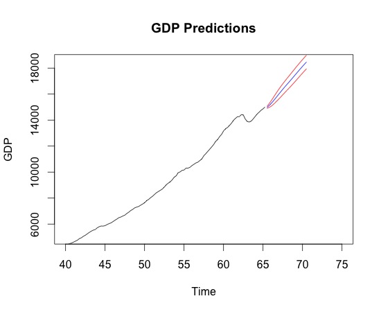
This code results in the following plot:

The blue line represents our point forecast and the red lines represent our 95% Confidence Level interval forecast.  I feel like the plot could be significantly cooler and therefore at its current appearance receives a 2 out of 10 for style.  It's bland, the x-axis doesn't have dates and there's not even any background color. If this plot had a name it would be doodoo.  A war must be fought against the army of lame plots.  Epic battles will proceed. Plots will be lost. Only one victor will stand.


Keep Dancin',

Steven J.

Assessing the Forecasting Ability of Our Model

Today we wish to see how our model would have faired forecasting the past 20 values of GDP. Why? Well ask yourself this: How can you know where your going, if you don't know where you've been? Once you understand please proceed on with the following post.

First recall the trend portion that we have already accounted for:


> t=(1:258)
> t2=t^2
> trendy= 892.656210 + -30.365580*t  + 0.335586*t2

And that the de-trended series is just that- the series minus the trend.

dt=GDP-trendy


As the following example will demonstrate- If we decide to assess the model with a forecast of the de-trended series alone we may come across some discouraging results:


> test.data<-dt[-c(239:258)]
> true.data<-dt[-c(1:238)]
> forecast.data<-predict(arima(test.data,order=c(10,0,0),include.mean=FALSE),n.ahead=20)$pred

Now we want to plot the forecast data vs. the actual values of the forecasted de-trended series to get a sense of whether this is accurate or not.

> plot(true.data,forecast.data)
> plot(true.data,forecast.data,main="True Data vs. Forecast data")

Clearly it appears as though there is little to no accuracy with the the forecast of our de-trended model alone.  In fact a linear regression of the forecast data on the true data makes this perfectly clear.

> reg.model<-lm(true.data~forecast.data)
> summary(reg.model)

Call:
lm(formula = true.data ~ forecast.data)

Residuals:
   Min     1Q Median     3Q    Max
-684.0 -449.0 -220.8  549.4  716.8

Coefficients:
                    Estimate    Std. Error    t value       Pr(>|t|)
(Intercept)   -2244.344   2058.828   -1.090         0.290
forecast.data     2.955      2.568         1.151         0.265

Residual standard error: 540.6 on 18 degrees of freedom
Multiple R-squared: 0.06851, Adjusted R-squared: 0.01676
F-statistic: 1.324 on 1 and 18 DF,  p-value: 0.265


> anova(reg.model)
Analysis of Variance Table

Response: true.data
                     Df  Sum Sq    Mean Sq   F value Pr(>F)
forecast.data  1     386920    386920      1.3238  0.265
Residuals     18    5260913  292273            


Now, is a good time to not be discouraged, but rather encouraged to add trend to our forecast.  When we run a linear regression of trend on GDP we quickly realize that 99.7 of the variance in GDP can be accounted for by the trend.


> reg.model2<-lm(GDP~trendy)
> summary(reg.model2)

Call:
lm(formula = GDP ~ trendy)

Residuals:
    Min      1Q  Median      3Q     Max
-625.43 -165.76  -36.73  163.04  796.33

Coefficients:
             Estimate Std. Error t value Pr(>|t|)  
(Intercept)  0.001371  21.870246     0.0        1  
trendy       1.000002   0.003445   290.3   <2e-16 ***
---
Signif. codes:  0 ‘***’ 0.001 ‘**’ 0.01 ‘*’ 0.05 ‘.’ 0.1 ‘ ’ 1

Residual standard error: 250.6 on 256 degrees of freedom
Multiple R-squared: 0.997, Adjusted R-squared: 0.997
F-statistic: 8.428e+04 on 1 and 256 DF,  p-value: < 2.2e-16

In the end we would have to had accounted for trend anyway so it just makes sense to use it when testing our models accuracy.  

> test.data1<-dt[-c(239:258)]  

# Important note is that the "-c(239:258)" includes everything except those particular 20 observations #

> true.data1<-dt[-c(1:238)]

> true.data2<-trendy[-c(1:238)]

> forecast.data1<-predict(arima(test.data1,order=c(10,0,0),include.mean=FALSE),n.ahead=20)$pred

> forecast.data2<-(true.data2)

> forecast.data3<-(forecast.data1+forecast.data2)

> true.data3<-(true.data1+true.data2)

Don't forget to plot your data:

> plot(true.data3,forecast.data3,main="True Values vs. Predicted Values")

...and regress the forecasted data on the actual data:

> reg.model3<-lm(true.data3~forecast.data3)

> summary(reg.model3)

Call:

lm(formula = true.data3 ~ forecast.data3)

Residuals:

   Min     1Q Median     3Q    Max 

-443.5 -184.2   16.0  228.3  334.8 

Coefficients:

                       Estimate          Std. Error      t-value    Pr(>|t|)    

(Intercept)        8.104e+03      1.141e+03   7.102       1.28e-06 ***

forecast.data3  4.098e-01        7.657e-02   5.352        4.37e-05 ***

---

Signif. codes:  0 ‘***’ 0.001 ‘**’ 0.01 ‘*’ 0.05 ‘.’ 0.1 ‘ ’ 1 

Residual standard error: 264.8 on 18 degrees of freedom

Multiple R-squared: 0.6141, Adjusted R-squared: 0.5926 

F-statistic: 28.64 on 1 and 18 DF,  p-value: 4.366e-05 

Looking at the plot and the regression results, I feel like this model is pretty accurate considering the fact this is a point forecast and not an interval forecast.  Next time on the Dancing Economist we will plot the forecasts into the future with 95% confidence intervals. Until then-

Keep Dancin'

Steven J

Forecasting In R: A New Hope with AR(10)

In our last post we determined that the ARIMA(2,2,2) model was just plain not going to work for us.  Although i didn't show its residuals failed to pass the acf and pacf test for white noise and the mean of its residuals was greater than three when it should have been much closer to zero.

Today we discover that an AR(10) of the de-trended GDP series may be the best option at hand.  Normally when we do model selection we start with the one that has the lowest AIC and then proceed to test the error terms (or residuals) for white noise. Lets take a look at the model specs for the AR(10):

> model7<-arima(dt,order=c(10,0,0))

> model7

Call:

arima(x = dt, order = c(10, 0, 0))

Coefficients:

         ar1      ar2            ar3       ar4           ar5     ar6           ar7      ar8        ar9     ar10

      1.5220  -0.4049  -0.2636  0.2360  -0.2132  0.1227  -0.0439  -0.0958  0.3244  -0.2255

s.e.  0.0604   0.1105   0.1131  0.1143   0.1154  0.1147   0.1139   0.1127  0.1111   0.0627

      intercept

       -21.6308

s.e.    57.5709

sigma^2 estimated as 1452:  log likelihood = -1307.76,  aic = 2639.52

The Ljung-Box Q test checks out to the 20th lag: 

> Box.test(model7$res,lag=20,type="Ljung-Box")

Box-Ljung test

data:  model7$res 

X-squared = 15.0909, df = 20, p-value = 0.7712

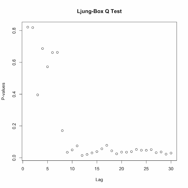
It even checks out to the 30th lag! I changed the way Iplotted the Ljung-Box Q values because after finding this little function called "LBQPlot" which makes life way easier.

> LBQPlot(model7$res,lag.max=30,StartLag=1)

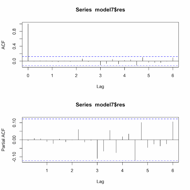
Most importantly both the ACF and the PACF of the residuals check out for the white noise process.  In the ARIMA(2,2,2) model these weren't even close to what we wanted them to be.

> par(mfrow=c(2,1))

> acf(model7$res)

> pacf(model7$res)

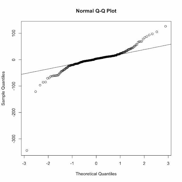
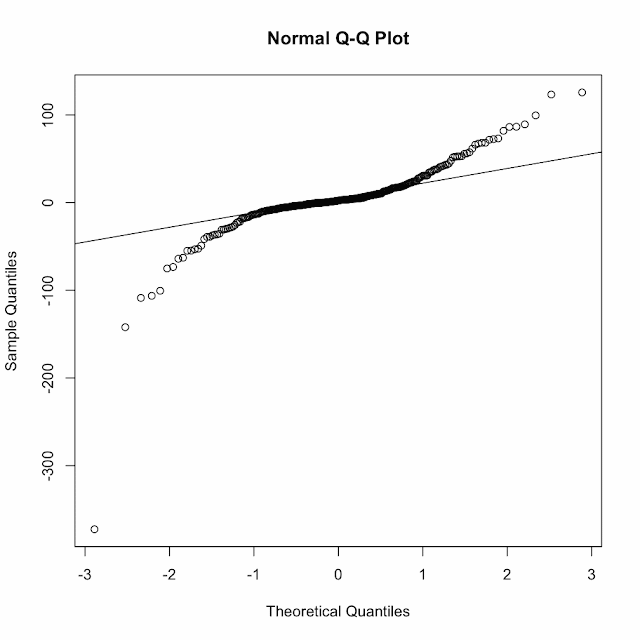
Unfortunately, our residuals continue to fail the formal tests for normality. I don't really know what to do about this or even what the proper explanation is, but I have a feeling that these tests are very very sensitive. 

> jarque.bera.test(model7$res)

Jarque Bera Test

data:  model7$res 

X-squared = 7507.325, df = 2, p-value < 2.2e-16

> shapiro.test(model7$res)

Shapiro-Wilk normality test

data:  model7$res 

W = 0.7873, p-value < 2.2e-16

The mean is also considerably closer to 0 but just not quite there.

> mean(model7$res)

[1] 0.7901055

Take a look at the plot for normality:

> qqnorm(model7$res)

> qqline(model7$res)

In the next post we are going to test how good our model actually is.  Today we found our optimal choice in terms of model specs, but we also should see how well it can forecast past values of GDP.  In addition to evaluating our models past accuracy we will also practice forecasting into the future.  As you continue to read these posts, you should be getting significantly better with R- I know I am!  We have covered many new codes that stem from many different libraries. I would like to keep on doing analysis in R so after we finish forecasting GDP I think I may move on to some Econometrics. Please keep forecasting and most certainly keep dancin',

Steven J.

Story of the Ljung-Box Blues: Progress Not Perfection

In the last post we determined that our ARIMA(2,2,2) model failed to pass the Ljung-Box test.  In todays post we seek to completely discredit the last posts claim and finally arrive at some needed closure.

The Ljung-Box is first performed on the series at hand, because it means that at least one of the autocorrelation functions is non zero. What does that mean?  Well, it means that we can forecast because the values in the series can be used to predict each other.  It helps us numerically come to the conclusion that the series itself is not a white noise process and so its movements are not completely random. 

When we perform the Ljung-Box in R on GDP we get the following results:

> Box.test(GDP,lag=20,type="Ljung-Box")

Box-Ljung test

data:  GDP 

X-squared = 4086.741, df = 20, p-value < 2.2e-16

What this output is telling us is to reject the null hypothesis that all of the autocorrelation functions out to 20 are zero.  At least one of these is non zero.  This gives us the green light to use AR, MA or ARMA in our approach towards modeling and forecasting.

The second time the Ljung-Box shows up is when we want to test to see if the error terms or residuals are white noise.  A good forecasting model will have to have zero correlation between its residuals or else you could forecast them.  It naturally follows that if you can forecast the error terms then a better model must exist.  

Here is the Ljung-Box Q test out to the 26th Lag:

> LjungBoxTest(res,k=2,StartLag=1)

  m    Qm     p-value:

  1  0.05     0.82118640

  2  0.05     0.81838128

  3  0.72     0.39541957

  4  0.75     0.68684256

  5  2.00     0.57224678

  6  2.41     0.66164894

  7  3.24     0.66255593

  8  9.05     0.17070965

  9 15.14    0.03429650

 10 15.54   0.04946816

 11 15.64   0.07487629

 12 22.14   0.01442010

 13 22.51    0.02073827

 14 22.72    0.03020402

 15 23.24    0.03889525

 16 23.24    0.05648292

 17 23.29    0.07809501

 18 26.81    0.04367819

 19 30.20    0.02494375

 20 30.20    0.03554725

 21 31.56    0.03500150

 22 32.46    0.03868275

 23 32.47    0.05241222

 24 34.14    0.04748629

 25 35.47    0.04672181

 26 36.28    0.05151986

As you can see with your very special eyes we fail to reject the null hypothesis out to the 8th lag.  So we have no evidence of residual autocorrelation and hence we have no evidence to contradict the assumption that the errors are white noise.  Our model checks out people!

Now if you want to plot the Ljung-Box just type in the following:

> x<-LjungBoxTest(res,k=2,StartLag=1)

> plot(x[,3],main="Ljung-Box Q Test",ylab="P-values",xlab="Lag")

The white noise process should also have a normal distribution with a mean of 0.  To do a rough test of normality we can run a simple Q-Q plot in R.  The values are normal if they rest on a line and aren't all over the place.

The following command gives us this plot:

qqnorm(res)
qqline(res)

The Q-Q plot seems to suggest normality- however there are some formal tests we can run in R to verify this assumption.  Two formal tests are the Jarque-Bera Test and the Shapiro-Wilk normality test.  Both have a null hypothesis that the series follows a normal distribution and therefore a rejection of the null suggests that the series does not follow a normal distribution.

> jarque.bera.test(res)

Jarque Bera Test

data:  res 

X-squared = 9660.355, df = 2, p-value < 2.2e-16

> shapiro.test(res)

Shapiro-Wilk normality test

data:  res 

W = 0.7513, p-value < 2.2e-16

Wow! Both of these test strongly reject the possibility of the white noise process having a normal distribution. 

We can still see if the mean of the residuals is zero by simply typing the following into R:

> mean(model$res)

[1] 3.754682

The mean is clearly not zero which implies we have some sort of a problem. In fact, it means that the Ljung-Box was not the proper test because it requires:

A. The time series be stationary
B. The white noise process has a normal distribution with mean zero.

Given that we just determined that the mean is definitely not zero and that both of our formal tests rejected the possibility of our white noise process following a normal distribution, we do indeed face a serious problem.  This is a evolving and growing period for us forecasting in R novices.  I don't have all the answers (clearly), but strides are made in the right direction every day. The greatest thing about making mistakes and tripping in the forest is getting back up and getting the hell out of there.  

Please keep posted and keep dancin',

Steven J.